Spin Angular Momentum
in Acoustic Field Theory
Justin Dressel
Chapman University crew: Lucas Burns, Derek White
Brown University crew: Tatsuya Daniel
RIKEN crew: Konstantin Bliokh, Franco Nori
ADVANCES IN OPERATOR THEORY WITH APPLICATIONS TO MATHEMATICAL PHYSICS
November 14, 2022
Acoustic Spin?
- Linear acoustic waves are longitudinal
- Usually described by a scalar potential field
- Scalar potential is dynamical in Lagrangian
-
Scalar fields can't have intrinsic spin
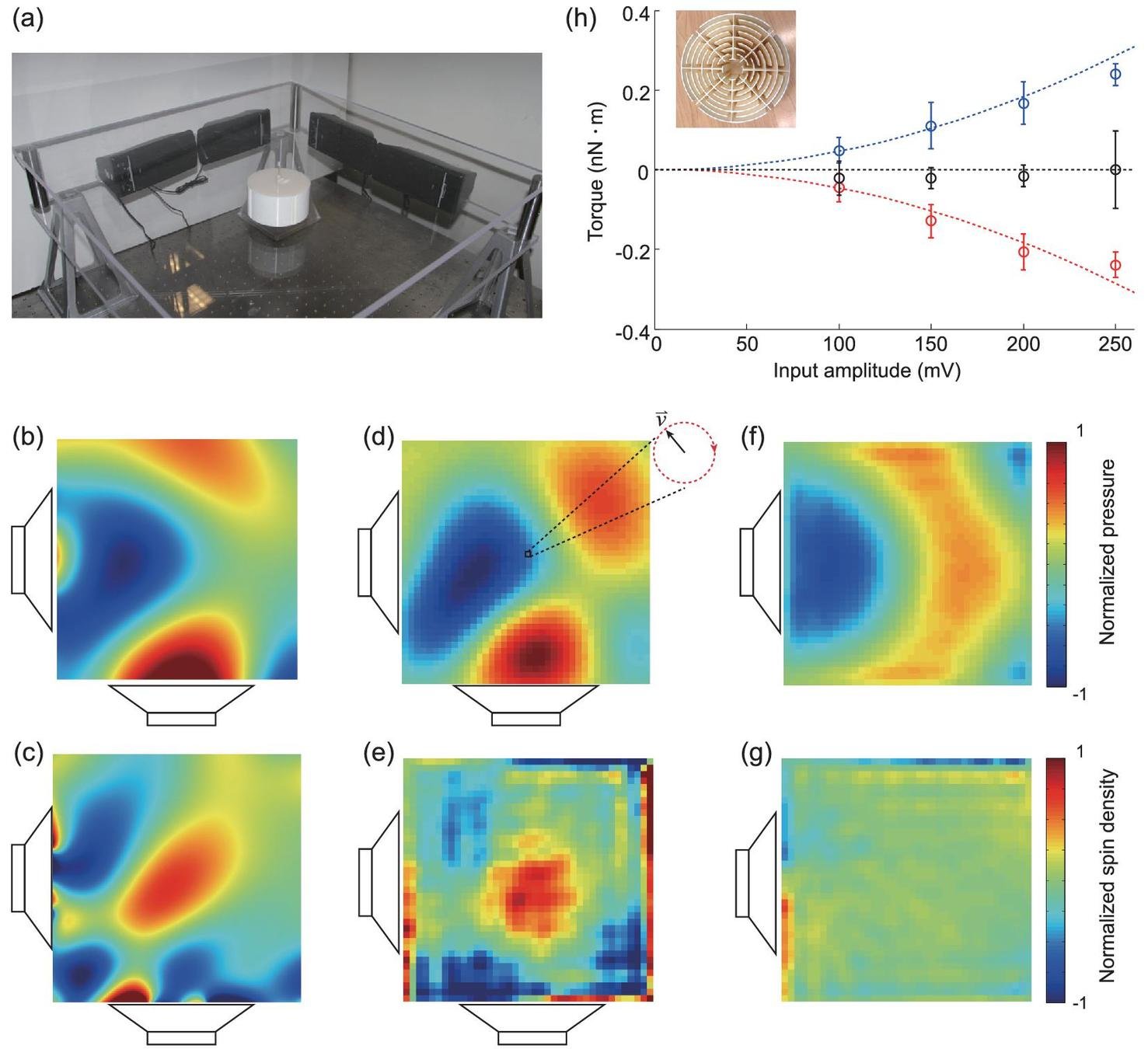
- In 2019 acoustic spin was measured!
- Acoustic velocity fields have a vector structure not in the scalar potential
- How do we understand this structure within Lagrangian field theory?
- Acoustic velocity fields have a vector structure not in the scalar potential
Shi et al. (2019) https://doi.org/10.1093/nsr/nwz059
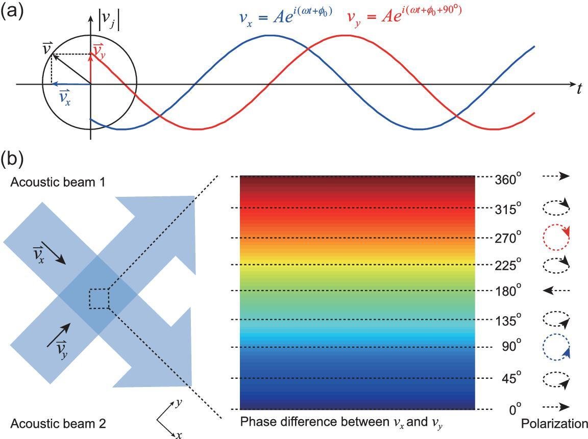
Acoustic Spin!
-
Microscopically, the origin of spin is clear:
- Superimposing two orthogonal longitudinal oscillations that are out of phase produces orbital molecular motion
- Coarse-graining the molecular motion
produces smooth effective field with
point-like angular momentum, i.e., spin
- Superimposing two orthogonal longitudinal oscillations that are out of phase produces orbital molecular motion
-
Pressure and Velocity fields have enough structure to describe the spin
- Strong analogies to electromagnetic fields
- But what is the dynamical potential field?
Shi et al. (2019) https://doi.org/10.1093/nsr/nwz059
Acoustic
Electromagnetic
\rho\,\partial_t \vec{v} = -\vec{\nabla} p
\beta\,\partial_t p = -\vec{\nabla}\cdot\vec{v}
\vec{\nabla}\times\vec{v} = \vec{0}
(Longitudinality)
\begin{aligned}
&\vec{v} : \text{velocity} \\
&p : \text{pressure}\\
&\rho : \text{mass density} \\
&\beta : \text{compressibility} \\
&c = \frac{1}{\sqrt{\rho\beta}} : \text{speed of sound}
\end{aligned}
\epsilon_0\,\partial_t \vec{E} = \vec{\nabla} \times \vec{H}
\mu_0\,\partial_t \vec{H} = -\vec{\nabla}\times \vec{E}
\vec{\nabla}\cdot\vec{E} = \vec{\nabla}\cdot\vec{H} = 0
(Transversality)
\begin{aligned}
&\vec{E} : \text{electric field}\\
&\vec{H} : \text{magnetic field} \\
&\epsilon_0 : \text{permittivity} \\
&\mu_0 : \text{permeability} \\
&c = \frac{1}{\sqrt{\epsilon_0\mu_0}} : \text{speed of light}
\end{aligned}
Source-free Equations of Motion
(Force / volume)
(Power / volume)
L \propto \frac{1}{2} \left[ \epsilon_0\,\vec{E}\cdot\vec{E} - \mu_0\,\vec{H}\cdot\vec{H} \right]
L \propto \frac{1}{2} \left[ \rho\,\vec{v}\cdot\vec{v} - \beta\,p^2 \right]
\sqrt{\epsilon_0}\vec{E} = -\partial_{ct}(\vec{A}_{e}/\sqrt{\mu_0}) - \vec{\nabla}(\sqrt{\epsilon_0}\phi_{e})
\sqrt{\mu_0}\,\vec{H} = \vec{\nabla}\times(\vec{A}_{e}/\sqrt{\mu_0})
\sqrt{\rho}\,\vec{v} = \vec{\nabla}(\phi/\sqrt{\rho})
\sqrt{\beta}\,p = -\partial_{ct}(\phi/\sqrt{\rho})
Need to introduce dynamical (scalar) potential \(\phi\):
\rho\,\partial_t \vec{v} = -\vec{\nabla} p
\beta\,\partial_t p = -\vec{\nabla}\cdot\vec{v}
\vec{\nabla}\times\vec{v} = \vec{0}
\epsilon_0\,\partial_t \vec{E} = \vec{\nabla} \times \vec{H}
\mu_0\,\partial_t \vec{H} = -\vec{\nabla}\times \vec{E}
\vec{\nabla}\cdot\vec{E} = 0
Dynamical Potential Fields
Acoustic
Electromagnetic
Fields \(\vec{v}\) and \(p\) are not the dynamical fields
L \propto \frac{1}{2\rho} \left[\vec{\nabla}\phi\cdot\vec{\nabla}\phi - (\partial_{ct}\phi)^2 \right]
Lagrangian formalism then produces correct equations of motion by varying \(\phi\):
Need to introduce dynamical potentials \((\phi_e,\vec{A}_e)\):
Fields \(\vec{E}\) and \(\vec{H}\) are not the dynamical fields
Lagrangian formalism then produces correct equations of motion by varying \((\phi_e,\vec{A}_e)\):
\vec{\nabla}\cdot\vec{H} = 0
L \propto \frac{1}{2} \left[ \rho\,\vec{v}\cdot\vec{v} - \beta\,p^2 \right] = \frac{1}{2\rho} \left[ \vec{\nabla}\phi\cdot\vec{\nabla}\phi - (\partial_{ct}\phi)^2 \right]
\rho\,\vec{v} = \vec{\nabla}\phi
p = -\partial_t\phi
\implies \rho\,\partial_t \vec{v} = -\vec{\nabla} p
\implies \partial_{ct} (p/c) +\vec{\nabla}\cdot(\rho\vec{v}) = 0
\implies \vec{\nabla}\times\vec{v} = \vec{0}
Potential Equations of Motion
Acoustic
[\partial_{ct}^2 - |\vec{\nabla}|^2]\phi = 0
Potential definitions imply two constraint equations:
Lagrangian variation produces wave equation of motion:
This equation enforces energy-momentum continuity.
L \propto \frac{1}{2} \left[ \epsilon_0\,\vec{E}\cdot\vec{E} - \mu_0\,\vec{H}\cdot\vec{H} \right]
\vec{E} = -\partial_t\vec{A}_{e} - \vec{\nabla}\phi_{e}
\mu_0\,\vec{H} = \vec{\nabla}\times\vec{A}_{e}
\epsilon_0\,\partial_t \vec{E} = \vec{\nabla} \times \vec{H}
\implies \mu_0\,\partial_t \vec{H} = -\vec{\nabla}\times \vec{E}
\implies \vec{\nabla}\cdot\vec{E} = 0
Electromagnetic
\implies \vec{\nabla}\cdot\vec{H} = 0
Potential definitions imply two constraint equations:
Lagrangian variation produces (wave) equations of motion:
[\partial_{ct}^2 - |\vec{\nabla}|^2]\phi_e = 0
[\partial_{ct}^2 - |\vec{\nabla}|^2]\vec{A}_e = 0
Potentials \((\phi_e,\vec{A}_e)\) have units (energy, momentum) / charge and have "gauge freedom": \((\phi_e,\vec{A})\mapsto (\phi_e - \partial_t \lambda, \vec{A} + \vec{\nabla}\lambda)\)
Lorenz-FitzGerald condition enforces energy-momentum continuity: \( \partial_{ct}(\phi_e/c) + \vec{\nabla}\cdot\vec{A}_e = 0\)
The potential \(\phi\) has units of (action / volume)
and has a "gauge freedom": \(\phi \mapsto \phi + \phi_0\)
The Spin Problem
A scalar potential \(\phi\) does not have enough structure to describe the observed acoustic spin!
\displaystyle \vec{S}_e = \frac{\sqrt{\varepsilon_0}}{c}\vec{E}\times\vec{A}_e
\displaystyle \vec{S} = \vec{0}
In Electromagnetism, the spin density computed using the Lagrangian formalism is potential-dependent:
In Acoustics, performing the same computation yields a vanishing spin density with potential \(\phi\):
This clearly contradicts experiment!
So how do we fix this problem theoretically?
Acoustics so Far
Examine the similarities to electromagnetism
But note the important differences:
- \((p,\,\vec{v})\) is 1+3 dimensions
- involved in stress-energy tensor
- not the dynamical field in Lagrangian
- 0 dimensional dynamical potential \(\phi\)
- \((\vec{E},\,\vec{H})\) is 3+3 dimensions
- involved in stress-energy tensor
- not the dynamical field in Lagrangian
- 1+3 dimensional dynamical potential \((\phi_e,\vec{A}_e)\)
- \((p,\, \vec{v})\) are longitudinal
- \((\vec{E},\,\vec{H})\) are transverse
- \(c\) is invariant speed of sound or light waves
\rho\,\partial_t \vec{v} = -\vec{\nabla} p
\beta\,\partial_t p = -\vec{\nabla}\cdot\vec{v}
\vec{\nabla}\times\vec{v} = \vec{0}
L \propto \frac{1}{2} \left[ \rho\,\vec{v}\cdot\vec{v} - \beta\,p^2 \right]
\rho\,\vec{v} = \vec{\nabla}\phi
p = -\partial_t\phi
(Lagrangian Density)
(Dynamical Scalar Potential)
What's missing?
Both theories have a Minkowski structure
- \((p/c,\,\vec{v})\) is 1+3 dimensional; \(\phi\) is 0 dimensional
-
structurally a spacetime 4-vector and scalar
-
- \((\vec{E},\,\vec{H})\) is 3+3 dimensions; \((\phi_e/c,\vec{A}_e)\) is 1+3 dimensional
-
structurally a spacetime bivector and 4-vector
-
structurally a spacetime bivector and 4-vector
- Motivated to construct "Acoustic Spacetime" by replacing speed of light with speed of sound
- Same Lorentz metric and tangent Clifford algebra
Signature: \((+---)\) Algebra: \(\text{Cl}_{1,3}(\mathbb{R})\)
- Structure is much easier to understand when expressed geometrically in 4D
(p/c, \rho\,\vec{v}) = (-\partial_{ct}\phi, \vec{\nabla}\phi)
\implies \partial_{ct} (p/c) +\vec{\nabla}\cdot(\rho\vec{v}) = 0
[\partial_{ct}^2 - |\vec{\nabla}|^2]\phi = 0
Acoustics
(\phi_e/c, \vec{A})
\partial_{ct} (\phi_e/c) +\vec{\nabla}\cdot\vec{A} = 0
\implies [\partial_{ct}^2 - |\vec{\nabla}|^2]\phi_e = 0
Electromagnetism
[\partial_{ct}^2 - |\vec{\nabla}|^2]\vec{A}_e = 0
Energy-momentum per volume
Energy-momentum per charge
Slight Diversion
(algebra of "spacetime" 101)
Constructing "Acoustic Spacetime" Algebra
\text{Basis: } \gamma_0,\,\gamma_1,\,\gamma_2,\,\gamma_3
Minkowski Space \(\mathcal{M}_{1,3}(\mathbb{R})\) :
\displaystyle \begin{aligned}\eta(a+b,\,a+b) &= (a+b)^2 = a^2 + b^2 + ab + ba \\ &= \eta(a,a) + \eta(b,b) + 2\eta(a,b) \\ \\ \implies& \eta(a,b) \equiv \frac{ab + ba}{2} \equiv a\cdot b \end{aligned}
\gamma_0 \cdot \gamma_0 = 1
\gamma_k \cdot \gamma_k = -1
\gamma_\mu \cdot \gamma_\nu = \eta_{\mu\nu} = \eta(\gamma_\mu,\,\gamma_\nu)
Minkowski metric
(symmetric bilinear form)
Algebraic Axioms: \(a,b,c\in\mathcal{M}_{1,3}(\mathbb{R})\)
- Associativity
\(a(bc) = (ab)c\)
- Left Distributivity
\(a(b+c) = ab + ac\)
- Right Distributivity
\((b+c)a = ba + ca\)
- Contraction
\(a^2 = aa = \eta(a,\,a)\)
Axioms constructively define Clifford algebra \( \text{Cl}_{1,3}(\mathbb{R}) \)
\displaystyle ab = \frac{ab + ba}{2} + \frac{ab - ba}{2} \equiv a\cdot b + a\wedge b
Symmetric part of product encodes metric:
Anti-symmetric part encodes Grassman wedge product:
(others zero)
(same as for differential forms)
Graded Clifford Basis (Dirac Algebra)
- (contravariant) basis:
\gamma_0\gamma_1\gamma_2\gamma_3
\gamma_1\gamma_0 \quad \gamma_2\gamma_0 \quad \gamma_3\gamma_0 \quad | \quad \gamma_1\gamma_2 \quad \gamma_2\gamma_3 \quad \gamma_3\gamma_1
\gamma_0 \quad | \quad \gamma_1 \quad \gamma_2 \quad \gamma_3
1
Grade
0
1
2
3
\gamma_\mu\gamma_\nu = \begin{cases}-\gamma_\nu\gamma_\mu = \gamma_\mu\wedge\gamma_\nu, & \mu\neq\nu \\\quad\,\, \eta_{\mu\nu} = \gamma_\mu\cdot\gamma_\nu, & \mu = \nu \end{cases}
4
\gamma_1\gamma_2\gamma_3 \quad | \quad \gamma_0\gamma_2\gamma_3 \quad \gamma_0\gamma_1\gamma_3 \quad \gamma_0\gamma_1\gamma_2
2^4 = 16\;\text{dimensions}
Bivector Planes (of rotation):
3 hyperbolic | 3 elliptic
Vector Lines (of translation):
1 timelike | 3 spacelike
Scalar Points
Pseudovector Volumes:
1 spacelike | 3 timelike
Pseudoscalar 4-Volumes
Multivector: \( M = \langle M \rangle_0 + \langle M \rangle_1 + \langle M \rangle_2 + \langle M \rangle_3 + \langle M \rangle_4 \)
- Reciprocal/dual/covariant basis:
\gamma^\mu \equiv (\gamma_\mu)^{-1} = \gamma_\mu / (\gamma_\mu)^2
Relative Frame Simplification (Pauli Algebra)
I
\vec{\sigma}_1 \quad \vec{\sigma}_2 \quad \vec{\sigma}_3 \quad | \quad I\vec{\sigma}_1 \quad I\vec{\sigma}_2 \quad I\vec{\sigma}_3
\gamma_0 \quad | \quad \gamma_1 \quad \gamma_2 \quad \gamma_3
1
0
1
2
3
I \equiv \gamma_0\gamma_1\gamma_2\gamma_3 \equiv \vec{\sigma}_1\vec{\sigma}_2\vec{\sigma}_3
(Spacetime-aware "imaginary unit" is the unit pseudoscalar: \(I^2 = -1\))
(commutes with even grade, anti-commutes with odd grade)
4
I\gamma_0 \quad | \quad I\gamma_1 \quad I\gamma_2 \quad I\gamma_3
Relative 3D space embedded as even-graded subspace:
\( \text{Cl}_{3,0}(\mathbb{R}) \)
Equivalent to complexified
3-vector (Pauli) algebra since \(I\) commutes with even grades
\vec{\sigma}_k \equiv \gamma_k\gamma_0 = \gamma_k \wedge \gamma_0
(Observed spatial directions in reference frame)
(Space axis dragged along temporal worldline)
Note duality transformation of left multiplication by \(-I\) : Hodge star operation \(\star\)
Multivector: \( M = [\alpha + (v_0 + \vec{v})\gamma_0 + \vec{A}] + I[\vec{B} + (w_0 + \vec{w})\gamma_0 + \beta] \)
Complex Structure & Spacetime Splits
Proper Form of Multivector:
\( M = \alpha + v + \mathbf{F} + Iw + I\beta = (\alpha + I\beta) + (v + Iw) + \mathbf{F} \)
Relative Frame Form of Multivector:
\( M = \alpha + (v_0 + \vec{v})\gamma_0 + (\vec{A} + I\vec{B}) + I(w_0 + \vec{w})\gamma_0 + I\beta \)
Components:
complex scalar
complex vector
bivector
scalar
polar paravector
polar vector
axial vector
axial paravector
pseudoscalar
4-vector
scalar
bivector
pseudovector
pseudoscalar
v = \sum_\mu v^\mu\gamma_\mu = \sum_\mu v_\mu \gamma^\mu = (v^0 + \sum_k v^k\vec{\sigma}_k)\gamma_0
\mathbf{F} = \sum_{\mu,\nu} F^{\mu\nu}\gamma_\mu\gamma_\nu = \sum_{\mu,\nu} F_{\mu\nu} \gamma^\mu\gamma^\nu = \sum_k A^k\vec{\sigma}_k + I\sum_k B^k\vec{\sigma}_k
4-vector components, or a scalar and a relative 3-vector
rank-2 antisymmetric tensor components, or a pair of 3-vectors (one polar, one axial)
Fields and Derivatives
Multivector field: (in tangent algebra at point \(x = (ct + \vec{x})\gamma_0 \) of flat Minkowski manifold)
\( M(x) = \alpha(x) + v(x) + \mathbf{F}(x) + Iw(x) + I\beta(x) \)
Vector derivative (Dirac differential operator):
3-Vector derivative (3-Gradient, Pauli differential operator):
\( \displaystyle \vec{\nabla} \equiv \gamma^0\wedge\nabla = \sum_k \vec{\sigma}^k \frac{\partial}{\partial x^k} \)
\( \vec{\nabla}\vec{v} = \vec{\nabla}\cdot\vec{v} + \vec{\nabla} \wedge \vec{v} = \vec{\nabla}\cdot\vec{v} + (\vec{\nabla}\times \vec{v})I \)
\displaystyle \nabla \equiv \sum_\mu \gamma^\mu \frac{\partial}{\partial x^\mu} = \gamma_0 \left[\frac{\partial}{\partial (ct)} + \vec{\nabla} \right] = \left[ \frac{\partial}{\partial (ct)} - \vec{\nabla} \right] \gamma_0
\displaystyle \nabla v \equiv \nabla \cdot v + \nabla \wedge v \Longleftrightarrow (\delta + d) v
(equivalent to co-differential \(\delta = \star^{-1}d\star\) plus exterior derivative \(d\) )
(contains both divergence and curl that lower and raise the grade)
\nabla^2 = \nabla\gamma_0^2\nabla = (\partial_{ct} - \vec{\nabla})(\partial_{ct} + \vec{\nabla}) = \partial^2_{ct} - \vec{\nabla}\cdot\vec{\nabla} \Longleftrightarrow d\delta + \delta d
(squares to Laplacian/d'Alembertian)
End Slight Diversion
(algebra of "spacetime" 101)
Maxwell's Equation (in concise spacetime algebra)
\mathbf{F}(x) = \sqrt{\epsilon_0}\sum_{k=1}^3E^k(x)\gamma_k\gamma_0 + \sqrt{\mu_0}I\sum_{k=1}^3 H^k(x) \gamma_k\gamma_0 = \sqrt{\epsilon_0}\vec{E}(x)+I\sqrt{\mu_0}\vec{H}(x)
\nabla \mathbf{F} = j
j = \sum_\mu j^\mu_e \gamma_\mu + \sum_\mu j^{\mu}_{m} \gamma_\mu I = j_e + j_m I = \sqrt{\mu_0}c(\rho_e + \vec{J}_e/c)\gamma_0 + \sqrt{\mu_0}(\rho_m + \vec{J}_m/c)\gamma_0 I
electric charge
density and current
This is Maxwell's Equation
\begin{aligned}
\nabla \mathbf{F} &= \sqrt{\epsilon_0}\gamma_0[(\vec{\nabla}\cdot\vec{E}) + (\partial_{ct}\vec{E}- \mu_0 c\vec{\nabla}\times\vec{H})] \\
&+ \sqrt{\epsilon_0}\gamma_0[\mu_0 c(\vec{\nabla}\cdot\vec{H}) + (\mu_0\partial_t\vec{H} + \vec{\nabla}\times\vec{E})]I \\
&= \sqrt{\mu_0}c\gamma_0(\rho_e - \vec{J}_e/c) + \sqrt{\mu_0}\gamma_0 (\rho_m - \vec{J}_m/c)I = j
\end{aligned}
Electromagnetic field bivector:
(Same form as complex Riemann-Silberstein 3-vector)
Electromagnetic source complex 4-vector:
magnetic charge
density and current
Contains all of the usual 3D Maxwell's Equations, and admits both electric and magnetic sources
\mathbf{G}(x) = \mathbf{F}(x)I^{-1} = \sqrt{\mu_0}\vec{H}(x) - I\sqrt{\epsilon_0}\vec{E}(x)
(dual field bivector)
\delta \mathbf{F} = j_e, \quad \delta \mathbf{G} = j_m \\
\mathbf{G} = \star\mathbf{F}, \quad \delta = \star^{-1}d\star
differential forms equivalent
Acoustic Equation (in concise spacetime algebra)
w(x) = \sqrt{\beta}\,p(x)\gamma_0 + \sqrt{\rho}\,\sum_{k=1}^3 v^k(x) \gamma_k = [\sqrt{\beta}\,p(x)+\sqrt{\rho}\,\vec{v}(x)]\gamma_0
\nabla w = \Lambda
\Lambda = \sqrt{\beta}\,g_0/c + \sqrt{\beta}\,\mathbf{G}_a = \sqrt{\beta}\,g_0/c + (\sqrt{\beta}\,\vec{g} + I\sqrt{\rho}\,\vec{h})
power
source
This is the Acoustic Equation
\begin{aligned}
\nabla w &= \nabla \cdot w + \nabla \wedge w \\
&= (\partial_{ct}\,p/c + \vec{\nabla}\cdot(\rho\vec{v}))/\sqrt{\rho} - \sqrt{\beta}(\partial_{ct}\,(\rho \vec{v}) + \vec{\nabla}p) + \sqrt{\rho}\vec{\nabla}\times\vec{v}I \\
&= \sqrt{\beta}g_0/c + \sqrt{\beta}\vec{g} + I \sqrt{\rho}\vec{h} = \Lambda
\end{aligned}
Velocity field 4-vector:
Acoustic source spinor (even-graded multivector):
force
source
Contains all of the pressure and velocity equations and admits all types of sources
\delta w = \sqrt{\beta}\, g_0/c, \quad d w = \sqrt{\beta}\,\mathbf{G}_a
differential forms equivalent
vorticity
source
equation admits a spinor source (scalar plus bivector)
Main structural difference from EM is that the acoustic velocity field is one grade lower
Poincare Lemma(s): Two Possible EM Potentials
\nabla \cdot \nabla \cdot (a_m I) = 0
\nabla \wedge \nabla \wedge a_e = 0
\begin{aligned}
&\text{if } \nabla \wedge \mathbf{F} = 0, \\ &\exists a_e: \mathbf{F} = \nabla \wedge a_e
\end{aligned}
"All exact forms are closed"
Poincare Lemma:
"All closed forms are exact."
(dda_e=0)
(d\mathbf{F} = 0 \implies \mathbf{F} = da_e)
(\delta\delta (\star^{-1} a_m)=0)
"All co-exact forms are co-closed"
\begin{aligned}
&\text{if } \nabla \cdot \mathbf{F} = 0, \\
&\exists (a_m I): \mathbf{F} = \nabla \cdot (a_m I) = (\nabla \wedge a_m)I
\end{aligned}
Dual Poincare Lemma:
"All co-closed forms are co-exact."
\begin{aligned}
(\delta \mathbf{F} = 0 \implies \mathbf{F} &= \delta (\star^{-1} a_m) \\
&= (\star^{-1} d \star)(\star^{-1} a_m) = \star^{-1} d a_m)
\end{aligned}
Electric Vector Potential Exists
Magnetic Pseudovector Potential Exists
(couples to electric sources)
(couples to magnetic sources)
Poincare Lemma(s): Two Possible Acoustic Potentials
\nabla \cdot \nabla \cdot \mathbf{A} = 0, \quad \mathbf{A} = \vec{a} + \vec{b}I
\nabla \wedge \nabla \phi = 0
\begin{aligned}
&\text{if } \nabla \wedge w = 0, \\ &\exists \phi: w = \nabla \phi
\end{aligned}
"All exact forms are closed"
Poincare Lemma:
"All closed forms are exact."
(dd\phi=0)
(dw = 0 \implies w = d\phi)
(\delta\delta (\star^{-1} \mathbf{A})=0)
"All co-exact forms are co-closed"
\begin{aligned}
&\text{if } \nabla \cdot w = 0, \\
&\exists \mathbf{A}: w = \nabla \cdot \mathbf{A}
\end{aligned}
Dual Poincare Lemma:
"All co-closed forms are co-exact."
\begin{aligned}
(\delta w = 0 \implies w &= \delta \mathbf{A})
\end{aligned}
Scalar Potential Exists
Bivector Potential Exists
(couples to power sources)
(couples to force and vorticity sources)
Gauge Freedom and Radiation Far-field
Acoustic Bivector Potential
\begin{aligned}
\mathbf{F} = \nabla \wedge a_e
\end{aligned}
Electric Vector Potential
Gauge freedom of a gradient
\begin{aligned}
a_e \mapsto a_e + \nabla \chi
\end{aligned}
\begin{aligned}
\nabla\mathbf{F} &= \nabla[\nabla \wedge (a_e + \nabla \chi)] \\
&= \nabla\cdot(\nabla \wedge a_e) = j_e
\end{aligned}
In a particular reference frame, can fully fix (Coulomb) gauge by enforcing transversality far from sources (radiation far-field)
Lorenz-FitzGerald condition yields wave equation
\begin{aligned}
\nabla \cdot a_e = 0 \implies \nabla^2 a_e = j_e
\end{aligned}
\begin{aligned}
a_e = (\phi_e/c + \vec{A}_e)\gamma_0, \quad \vec{\nabla}\cdot\vec{A}_e = \phi_e = 0
\end{aligned}
\begin{aligned}
\nabla \cdot a_e = 0 \implies \nabla^2 a_e = j_e
\end{aligned}
\begin{aligned}
w = \nabla \cdot \mathbf{A} &= \nabla \cdot (\vec{a} + \vec{b} I) \\
&= \gamma_0[(\vec{\nabla}\cdot\vec{a}) + (\partial_{ct}\vec{a}- \vec{\nabla}\times\vec{b})] \\
&= \gamma_0(\sqrt{\beta}\,p - \sqrt{\rho}\,\vec{v})
\end{aligned}
Gauge freedom of a curl
\begin{aligned}
\mathbf{A} \mapsto \mathbf{A} + \nabla\wedge \xi
\end{aligned}
\begin{aligned}
\nabla w &= \nabla[\nabla \cdot (\mathbf{A} + \nabla \wedge \xi)] \\
&= \nabla\wedge(\nabla \cdot \mathbf{A}) = \Lambda
\end{aligned}
Lorenz-FitzGerald-like condition yields wave equation
\begin{aligned}
\nabla \wedge \mathbf{A} = 0 \implies \nabla^2 \mathbf{A} = \mathbf{G}_a
\end{aligned}
In a particular reference frame, can fully fix (Coulomb-like) gauge by enforcing longitudinality and no vorticity far from sources
\begin{aligned}
\mathbf{A} = \vec{a} + \vec{b}I,\qquad \vec{\nabla}\times\vec{a} = \vec{b} = 0
\end{aligned}
Radiation Far-field Potential Meaning
Acoustic Bivector Potential
\begin{aligned}
\mathbf{F} = \nabla \wedge a_e
\end{aligned}
Electric Vector Potential
\begin{aligned}
\vec{\nabla}\cdot\vec{A}_e = \phi_e = 0
\end{aligned}
\begin{aligned}
\nabla \cdot a_e = 0 \implies \mathbf{F} = \nabla a_e
\end{aligned}
Lorenz-FitzGerald-like condition yields:
\begin{aligned}
\nabla \wedge \mathbf{A} = 0 \implies w = \nabla \mathbf{A}
\end{aligned}
The bivector potential has been fixed to a longitudinal 3-vector potential \(\vec{x} = -\sqrt{\beta}\,\vec{a}\) with units of mean molecular displacement
\begin{aligned}
\vec{\nabla}\times\vec{a} = \vec{b} = 0
\end{aligned}
Lorenz-FitzGerald condition yields:
Coulomb gauge far from sources yields:
\vec{E} = - \partial_t\vec{A}_e
\vec{H} = \vec{\nabla}\times\vec{A}_e
3-vector potential \(\vec{A}_e\) has units of field-momentum per unit charge
In this fixed gauge, the electric field is the rate at which momentum is removed from the field, while the magnetic field describes the circulation (vorticity) of that momentum
\begin{aligned}
w = \nabla \cdot \mathbf{A}
\end{aligned}
Coulomb-like gauge far from sources yields:
\begin{aligned}
p &= -(\vec{\nabla}\cdot\vec{x})/\beta \\
\vec{v} &= \partial_t\vec{x}
\end{aligned}
In this fixed gauge, the velocity field is the rate of change of the mean displacement field, while the pressure field is related to expansion and contraction via the compressibility of the fluid
Radiation Far-field Intrinsic Spin
Acoustic Bivector Potential
Electric Vector Potential
\begin{aligned}
\vec{\nabla}\cdot\vec{A}_e = \phi_e = 0
\end{aligned}
\begin{aligned}
\vec{\nabla}\times\vec{a} = \vec{b} = 0
\end{aligned}
Coulomb gauge with no sources:
\vec{E} = - \partial_t\vec{A}_e
\vec{H} = \vec{\nabla}\times\vec{A}_e
Derived spin-vector has the asymmetric form:
Coulomb-like gauge with no sources yields:
\begin{aligned}
p &= -(\vec{\nabla}\cdot\vec{x})/\beta \\
\vec{v} &= \partial_t \vec{x}
\end{aligned}
\vec{S} = \vec{E}\times\vec{A}_e
Magnetic Pseudovector Potential
\begin{aligned}
\vec{\nabla}\cdot\vec{C}_m = \phi_m = 0
\end{aligned}
\vec{E} = - \vec{\nabla}\times\vec{C}_m
\vec{H} = - \partial_t \vec{C}_m
Spin-vector has other asymmetric form:
\vec{S} = \vec{B}\times\vec{C}_m
Derived spin-vector has the asymmetric form:
\vec{S} = \vec{x} \times (\rho \vec{v})
\vec{x} = -\sqrt{\beta}\,\vec{a}
\rho\vec{v} = \vec{\nabla}\phi
p = -\partial_t\phi
Acoustic Scalar Potential
Spin-vector has other asymmetric form:
\vec{S} = \vec{0}
(angular momentum density!)
None of the Derived Spin Vectors are Correct!
Acoustic Bivector Potential
Electric Vector Potential
\vec{S} = \vec{E}\times\vec{A}_e
Magnetic Pseudovector Potential
\vec{S} = \vec{B}\times\vec{C}_m
\vec{S} = \vec{x} \times (\rho \vec{v})
Acoustic Scalar Potential
\vec{S} = \vec{0}
Correct (Measured) Spin Vector
\displaystyle \vec{S} = \frac{1}{2}\left[ \vec{E}\times\vec{A}_e + \vec{B}\times\vec{C}_m \right]
Correct (Measured) Spin Vector
\displaystyle \vec{S} = \frac{1}{2} \left[ \vec{x}\times(\rho \vec{v}) \right]
In both EM and Acoustics, the correct (measured) spin vector is the average of those derived from the two possible dynamical potentials!
How can we derive this from the field theory framework correctly?
[Toftul, Bliokh, Petrov, Nori, PRL. 123, 183901 (2019)]
[Bliokh et al. New J Phys 15, 033026 (2013)]
Dual-symmetry : Electric-Magnetic Egalitarianism
\mathbf{F}(x) = \mathbf{f}(x)\,e^{I\theta(x)/2} = \sqrt{\epsilon_0}\vec{E}(x)+I\sqrt{\mu_0}\vec{H}(x)
\nabla \mathbf{F} = j
j = j_e + j_m I = \sqrt{\epsilon_0}(\rho_e + \vec{J}_e/c)\gamma_0 + \sqrt{\mu_0}(\rho_m + \vec{J}_m/c)\gamma_0 I
\(\{\)
Complete EM dynamics:
A hidden gauge symmetry is now evident:
e^{-I\phi/2}\nabla \mathbf{F}e^{I\phi/2} = e^{-I\phi/2}je^{I\phi/2}
The pseudoscalar \(I\) generates phase rotations in the usual way:
this has the effect of swapping the electromagnetic fields and source charges
e^{-I\phi/2}\nabla \mathbf{F}e^{I\phi/2} = \nabla\left[e^{I\phi/2}\mathbf{F}e^{I\phi/2}\right] = \nabla \left[\mathbf{F}e^{I\phi}\right] = \nabla \left[ (\cos\phi\,\vec{E} - \sin\phi\,\vec{B}) + (\sin\phi\,\vec{E} + \cos\phi\,\vec{B})I\right] = \nabla(\vec{E}' + \vec{B}'I)
e^{-I\phi/2}je^{I\phi/2} = je^{I\phi} = (\cos\phi\,j_e - \sin\phi\,j_m) + (\sin\phi\,j_e + \cos\phi\,j_m)I = j_e' + j_m'I
Physics is the same provided that both source and field definitions are changed in tandem
Can always choose \(\phi\) to make all charges electric (\(j'_m = 0\))
Vacuum fields far from sources (\(j = 0\)) always have this field-exchange symmetry
Electromagnetic Complex Vector Potential
\mathbf{F}(x) = \nabla z(x)
Postulate vector potential:
z(x) = \displaystyle \frac{a_e(x) + a_m(x)I}{\sqrt{2}}
Must be complex potential to satisfy dual symmetry
\mathbf{F} = \displaystyle \frac{\mathbf{F}_e + \mathbf{G}_m I}{\sqrt{2}} = \frac{\nabla \wedge a_e + \nabla \cdot (a_mI)}{\sqrt{2}}
0 = \nabla \cdot a_e = \nabla\cdot a_m
Lorenz-Fitzgerald conditions assumed
\mathbf{F} = \vec{E} + \vec{H}I \qquad a_e = (\phi_e + \vec{A}_e)\gamma_0 \qquad a_m = (\phi_m + \vec{C}_m)\gamma_0
\vec{E} = \displaystyle \frac{-\vec{\nabla}\phi_e - \partial_{ct}\vec{A}_e - \vec{\nabla}\times\vec{C}_m}{\sqrt{2}}
\vec{H} = \displaystyle \frac{-\vec{\nabla}\phi_m - \partial_{ct}\vec{C}_m + \vec{\nabla}\times\vec{A}_e}{\sqrt{2}}
Relative EM fields regain symmetry in definitions
\implies \nabla\mathbf{F}(x) = \nabla^2 z(x) = j(x)
Obvious wave equation
Electric and Magnetic potentials
contribute equally
(special case of Hodge Decomposition)
Dual-Symmetric Electromagnetic Lagrangian
L[z,\tilde{z}] = \displaystyle \frac{(\nabla z)\cdot(\nabla \tilde{z})}{2} = \frac{\mathbf{F} \cdot \mathbf{F}_{\rm conj}}{2} \neq \frac{\mathbf{F}\cdot\mathbf{F}}{2}
Must consider complex vector potential and its conjugate
z = \displaystyle \frac{a_e + a_m I}{\sqrt{2}}
\tilde{z} = \displaystyle \frac{a_e - a_m I}{\sqrt{2}}
Much like done with complex scalar potentials,
the Lagrangian must be varied with respect to
both \(z\) and \(\tilde{z}\) to get the correct result
\nabla^2 z = \displaystyle \frac{\nabla^2 a_e + \nabla^2 (a_m I)}{\sqrt{2}} = \nabla\mathbf{F} = 0
\nabla^2 \tilde{z} = \displaystyle \frac{\nabla(\nabla a_e - \nabla (a_m I))}{\sqrt{2}} = \nabla \mathbf{F}_{\rm conj} = 0
The first equation yields Maxwell's equation,
while the second forces each potential contribution to the total measured fields to be exactly equal
In the presence of sources, the conjugate field acquires nontrivial equations of motion that steer the measured field into a biased potential representation. This mechanism automatically locks the potential representation to match the source.
Noether's Theorem and EM Dual Symmetry
e^{-I\phi/2}\nabla \mathbf{F}e^{I\phi/2} = e^{-I\phi/2}je^{I\phi/2}
The global phase gauge symmetry leads to an independently conserved quantity
\underline{X}(I) = [\chi I + \vec{S}I^{-1}]\gamma_0
Helicity pseudocurrent is conserved Noether charge
\chi = \displaystyle \frac{\vec{B} \cdot \vec{A}_e - \vec{E} \cdot \vec{C}_m}{2}
\vec{S} = \displaystyle \frac{\vec{E}\times\vec{A}_e + \vec{B}\times \vec{C}_m}{2}
Correct spin-density pseudovector is the helicity flux density
Correct helicity-density pseudoscalar is also obtained
These definitions only make sense when properly dual-symmetric fields are used
They match measurements only with full electric-magnetic potential symmetry
Acoustic Spinor Potential
w(x) = \nabla \psi(x)
Postulate spinor potential:
\psi(x) = \displaystyle \frac{\phi'(x) + \mathbf{A}(x)}{\sqrt{2}}
Combines both scalar and bivector potentials in similar manner to the complex vector EM potential
w = \displaystyle \frac{w_\phi + w_\mathbf{A}}{\sqrt{2}} = \frac{\nabla \wedge \phi' + \nabla \cdot \mathbf{A}}{\sqrt{2}}
0 = \nabla \wedge \mathbf{A}
Lorenz-Fitzgerald-like condition assumed
w = (\sqrt{\beta}\,p + \sqrt{\rho}\,\vec{v})\gamma_0 \quad \mathbf{A} = -\vec{x}/\sqrt{\beta} + I\,\vec{b}/\sqrt{\rho} \quad \phi' = \sqrt{\rho}\,\phi
p = \displaystyle \frac{- \partial_t\phi' - (\vec{\nabla}\cdot\vec{x})/\beta}{\sqrt{2}}
\vec{v} = \displaystyle \frac{\vec{\nabla}(\phi'/\rho) + \partial_t\vec{x} + \vec{\nabla}\times(\vec{b}/\rho)}{\sqrt{2}}
Pressure and velocity
definitions become
symmetric
\implies \nabla v(x) = \nabla^2 \psi(x) = \Lambda(x)
Obvious spinor wave equation
Scalar and Bivector potentials
contribute equally
(special case of Hodge decomposition)
Acoustic Spinor Lagrangian
L[\psi,\tilde{\psi}] = \displaystyle \frac{(\nabla \psi)\cdot(\nabla \tilde{\psi})}{2} = \frac{\mathbf{w} \cdot \mathbf{w}_{\rm conj}}{2} \neq \frac{\mathbf{w}\cdot\mathbf{w}}{2}
Must consider spinor potential and its conjugate
\psi = \displaystyle \frac{\phi + \mathbf{A}}{\sqrt{2}}
\tilde{\psi} = \displaystyle \frac{\phi - \mathbf{A}}{\sqrt{2}}
Must be varied with respect to
both \(\psi\) and \(\tilde{\psi}\) to get the correct result
\nabla^2 \psi = \displaystyle \frac{\nabla^2 \phi + \nabla^2 \mathbf{A}}{\sqrt{2}} = \nabla w = 0
\nabla^2 \tilde{\psi} = \displaystyle \frac{\nabla(\nabla \phi - \nabla \mathbf{A})}{\sqrt{2}} = \nabla w_{\rm conj} = 0
The first equation yields the acoustic equation,
while the second forces each potential contribution to the total measured fields to be exactly equal
In the presence of sources, the conjugate field acquires nontrivial equations of motion that steer the measured field into a biased potential representation. This mechanism automatically locks the potential representation to match the source.
Finally, the Acoustic Field Spins Correctly!
\vec{S} = \displaystyle \frac{\vec{x} \times (\rho\vec{v})}{2}
Correct spin-density pseudovector
The correctly measured value of the far-field (source-free) spin-density is only obtained with symmetric potentials
\bar{\vec{S}} \to \displaystyle \frac{\rho\,\text{Im}(\vec{v}^*\times\vec{v})}{4\omega}
Monochromatic field cycle-average
Conclusions
- Acoustic fields can carry intrinsic spin, and we can now derive it!
- Spacetime Clifford algebra is a very convenient mathematical language
- The dual-symmetric structure of the electromagnetic theory becomes manifest when expressed in geometrically invariant forms
- The conserved quantity from Noether's theorem resulting from the continuous dual-symmetry in vacuum field propagation is the helicity
- A similarly symmetric spinor potential is needed in acoustics to correctly derive the spin density as part of a conserved Noether current
Thank you!
JD, Bliokh, Nori, Physics Reports 589 1-71 (2015)
Burns, Bliokh, Nori, JD, New J Physics 22 053050 (2020)
Spin Angular Momentum in Acoustic Field Theory
By Justin Dressel
Spin Angular Momentum in Acoustic Field Theory
ADVANCES IN OPERATOR THEORY WITH APPLICATIONS TO MATHEMATICAL PHYSICS, November 14, 2022. Using an acoustic analog of Minkowski geometry, we construct a Lagrangian representation of acoustic field theory that accounts for the recently measured nonzero spin-angular-momentum density of sound fields in fluids or gases. While the traditional acoustic Lagrangian representation of the measured pressure and velocity fields using a dynamical scalar potential is unable to describe the vector character of the spin, we show that the pressure-velocity 4-vector additionally admits a dynamical bivector potential that correctly accounts for the spin. In the equilibrium frame this bivector potential reduces to a displacement field with amplitude equal to the scalar potential, such that its gauge freedom is equivalent to the arbitrary choice of displacement origin. The two potentials combine into an even-graded spinor potential with dynamics that recover the observed local radiation forces and torques on small probe particles, as well as the correct canonically conserved momentum and spin densities as proper Noether currents. This twin-potential construction for acoustics closely mirrors a formulation of vacuum electromagnetism that combines both electric- and magnetic-potential representations into a manifestly dual-symmetric odd-graded potential.


