Optical Ventriloquism
and Local Streamlines
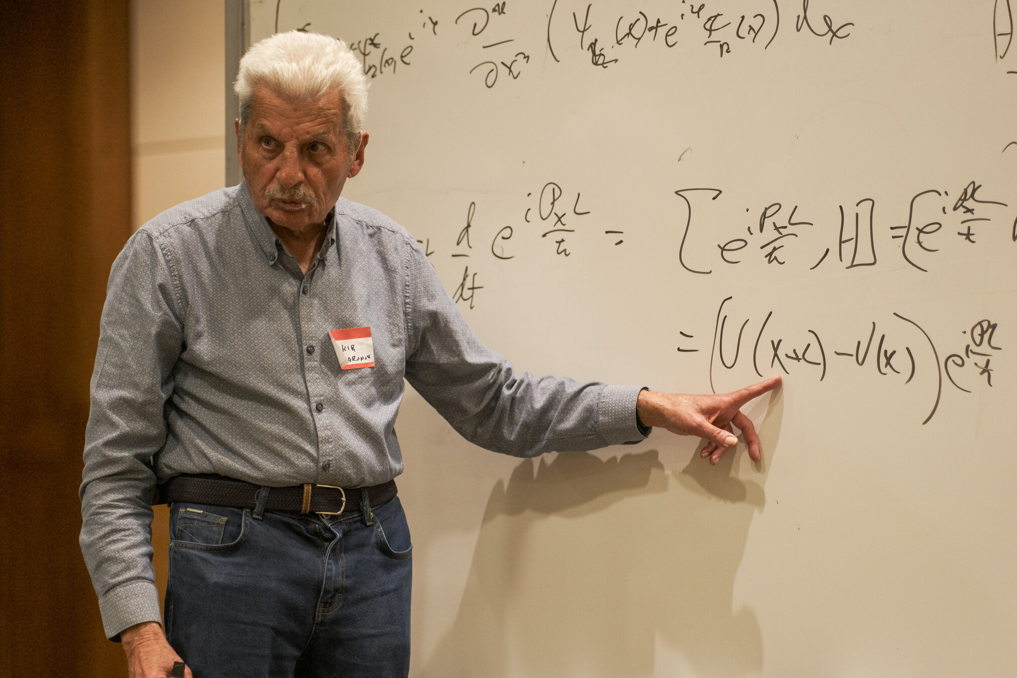
Justin Dressel
Institute for Quantum Studies, Chapman University
Superoscillations Conference, Cetraro 2024
Super-oscillations
"You can locally find frequencies outside the band limits of a signal."
-- Yakir Aharonov (paraphrased)
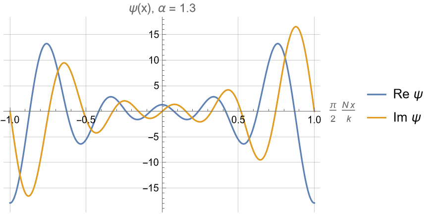
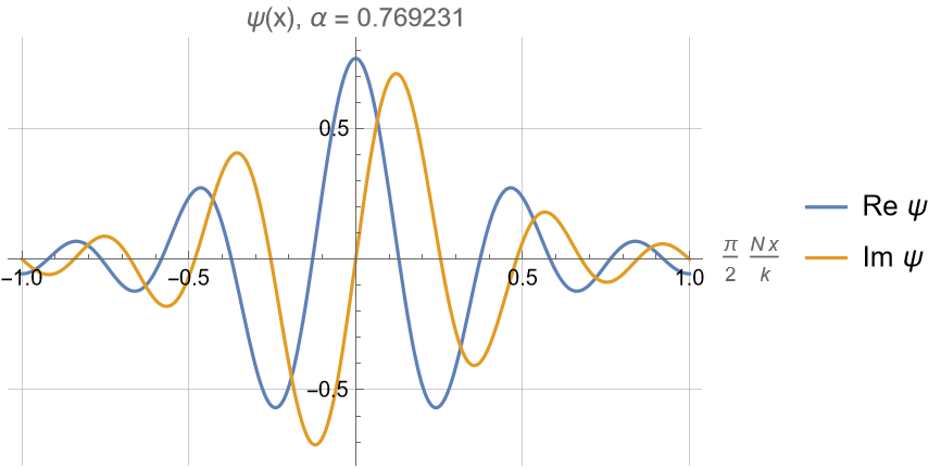
Consider the following wave function
(resulting after N steps of a binary quantum walk):
\begin{aligned}\psi(x) &= [\cos(kx/N) + i\alpha\sin(kx/N)]^N \\
&= \left[\frac{1+\alpha}{2}e^{ikx/N} + \frac{1-\alpha}{2}e^{-ikx/N}\right]^N = \sum_{n=0}^N c_n e^{ik_nx} \\
k_n &= (2n/N-1)k \in [-k,k]
\end{aligned}
Wave numbers band-limited
Super-oscillations
For small \(kx/N\), this simplifies:
\begin{aligned}\psi(x) &= \left[\frac{1+\alpha}{2}e^{ikx/N} + \frac{1-\alpha}{2}e^{-ikx/N}\right]^N \\
&\approx \left[\frac{1+\alpha}{2}(1+ikx/N+\cdots) + \frac{1-\alpha}{2}(1-ikx/N+\cdots)\right]^N \\
&\approx \left[1 + \alpha(ikx/N)+\cdots \right]^N \approx e^{i\alpha kx}
\end{aligned}
Physicist's interest:
Near \(x=0\) the function \(\psi(x)\) locally looks like a wave with scaled wavenumber \(\alpha k\).
This local wavenumber can be outside the band limits \(k_n \in [-k,k]\) for \(\alpha > 1\)!
Mathematician's interest:
In the limit \(N\to\infty\), the whole function \(\psi(x)\) converges to \(e^{i\alpha kx}\) everywhere.
Super-oscillation: Weak Value Perspective
The local wavenumber \(k_{\rm eff}(x)\) gives the local mean momentum:
\begin{aligned}p(x) &= \hbar k_{\rm eff}(x) \equiv \frac{-i\hbar \partial_x \psi(x)}{\psi(x)} = \frac{\langle x|\hat{p}|\psi\rangle}{\langle x | \psi\rangle} \\
%&= k\frac{\frac{1+\alpha}{2}e^{ikx/N} - \frac{1-\alpha}{2}e^{-ikx/N}}{\frac{1+\alpha}{2}e^{ikx/N} + \frac{1-\alpha}{2}e^{-ikx/N}}
%&= k\frac{\alpha \cos(kx/N) + i\sin(kx/N)}{\cos(kx/N) + i\alpha\sin(kx/N)} \\
\end{aligned}
\begin{aligned}
p(x) &= p_{\rm Bohm}(x) + i\, p_{\rm Nelson}(x)
\end{aligned}
This is a weak value of the momentum operator \(\hat{p}\), conditioned on \(x\)
It is generally complex:
- Real part: Bohmian momentum
- Imaginary part: Nelsonian "osmotic" momentum
\begin{aligned}
\psi(x) &\equiv \sqrt{\rho(x)}e^{iS(x)/\hbar} \implies
\begin{cases}
p_{\rm Bohm} = \partial_x S(x) \\
p_{\rm Nelson} = -\frac{1}{2}\partial_x \ln\rho(x)
\end{cases}
\end{aligned}
Rate of phase change
Rate of exponential growth/decay
\begin{aligned}\psi(x) &= \left[\cos(kx/N) + i\alpha\sin(kx/N)\right]^N
\end{aligned}
\begin{aligned}
p(x) &= -i\hbar\partial_x\ln\psi(x) = \hbar k_{\rm eff}(x) \equiv \hbar k\, n(x)
\end{aligned}
The local wave number has a complex refractive index:
Super-oscillation: Refractive Index
For the standard super-oscillating wave function:
\begin{aligned}
n(x) \equiv &\frac{\alpha + i \tan(kx/N)}{1 + i\alpha \tan(kx/N)} = n_r(x) + i n_i(x)
\end{aligned}
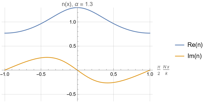
Real and imaginary parts are Hilbert transforms
of each other (Kramers-Kroenig relation)
Similar complex structure to a resonance linewidth
Super-oscillatory Refractive Index
\begin{aligned}
\displaystyle \frac{p(x)}{\alpha \hbar k} = &\frac{1 + i(1/\alpha) \tan(kx/N)}{1 + i\alpha \tan(kx/N)} \\
\xrightarrow{kx/N\to 0} \quad &1 + i\frac{kx}{N}\frac{1 - \alpha^2}{\alpha}
\end{aligned}
Superoscillatory region near \(x\approx 0\) looks like a resonance feature of \(n(x)\).
Limit of \(N\to\infty\) only rescales \(x\) to zoom in to center of the resonance peak.
For \(\alpha \geq 1\) :
Super-oscillatory Refractive Index
\begin{aligned}
\displaystyle \frac{\alpha p(x)}{\hbar k} = &\frac{\alpha^2 + i\alpha \tan(kx/N)}{1 + i\alpha \tan(kx/N)} \\
\xrightarrow{kx/N\to \pi/2} \quad &1 + i\left(\frac{kx}{N}-\frac{\pi}{2}\right)\left(\alpha - \frac{1}{\alpha}\right)
\end{aligned}
For \(-1\leq \alpha \leq 1\) :
Superoscillatory region near \(kx/N \approx \pm \pi/2\) still looks like a resonance feature of \(n(x)\).
Limit of \(N\to\infty\) pushes peak out to infinity.
Super-positions
"You can arrange for a point to look like it was in a different position than it actually was."
-- Yakir Aharonov (paraphrased)
Consider the same function but in Fourier space:
\begin{aligned}\tilde{g}(k) &= \sum_{n=0}^N c_n e^{-2\pi ik (x-x_n)}, \quad
x_n = (2n/N -1)x_0 \\
g(x) &= \mathcal{F}^{-1}\tilde{g}(k) = \sum_{n=0}^N c_n \delta(x - x_n)
\end{aligned}
After a Fourier transform, it looks like a set of point positions within a bounded region: \(x_n \in [-x_0, x_0]\)
Super-positions
Following exactly the same argument as before:
\begin{aligned}\tilde{g}(k) &= \sum_{n=0}^N c_n e^{-2\pi ik (x-x_n)} \approx e^{-2\pi ik(x - \alpha x_0)} \\
g(x) &= \mathcal{F}^{-1}\tilde{g}(k) \approx \delta(x - \alpha x_0)
\end{aligned}
After a Fourier transform, the function \(g(x)\) approximates a point position \(\alpha x_0\) when \(kx_0/N \to 0\).
\(\alpha x_0\) can be outside the bounded region \([-x_0,x_0]\), meaning the position seems to be where it isn't!
Laboratory Super-positions?
\begin{aligned}\tilde{g}(k) &= \sum_{n=0}^N c_n e^{-2\pi ik (x-x_n)} \approx e^{-2\pi ik(x - \alpha x_0)} \\
g(x) &= \mathcal{F}^{-1}\tilde{g}(k) \approx \delta(x - \alpha x_0)
\end{aligned}
But how to show this dual superoscillation effect experimentally?
The condition \(kx_0/N \approx 0\) suggests a post-selection to \(k\approx 0\).
This idea is natural for paraxial beam propagation.
Laboratory Super-positions?
For the initial beam profile, the (transverse) position weak value
\begin{aligned}x(p) &\equiv \frac{i\hbar \partial_p \tilde{\psi}(p)}{\tilde{\psi}(p)} = \frac{\langle p|\hat{x}|\psi\rangle}{\langle p | \psi\rangle}
%&= k\frac{\frac{1+\alpha}{2}e^{ikx/N} - \frac{1-\alpha}{2}e^{-ikx/N}}{\frac{1+\alpha}{2}e^{ikx/N} + \frac{1-\alpha}{2}e^{-ikx/N}}
%&= k\frac{\alpha \cos(kx/N) + i\sin(kx/N)}{\cos(kx/N) + i\alpha\sin(kx/N)} \\
\end{aligned}
approximates \(\alpha x_0\) when the (transverse) momentum \(p \approx 0\).
After propagation to the far field, one should thus find
that locally \(p\approx 0\) near transverse position \(\alpha x_0\) to be consistent.
So in far field put a pinhole at \(\alpha x_0\) and measure the local \(p(x)\).
If \(p(\alpha x_0)\approx 0\) then it looks like straight ray propagation from \(\alpha x_0\).
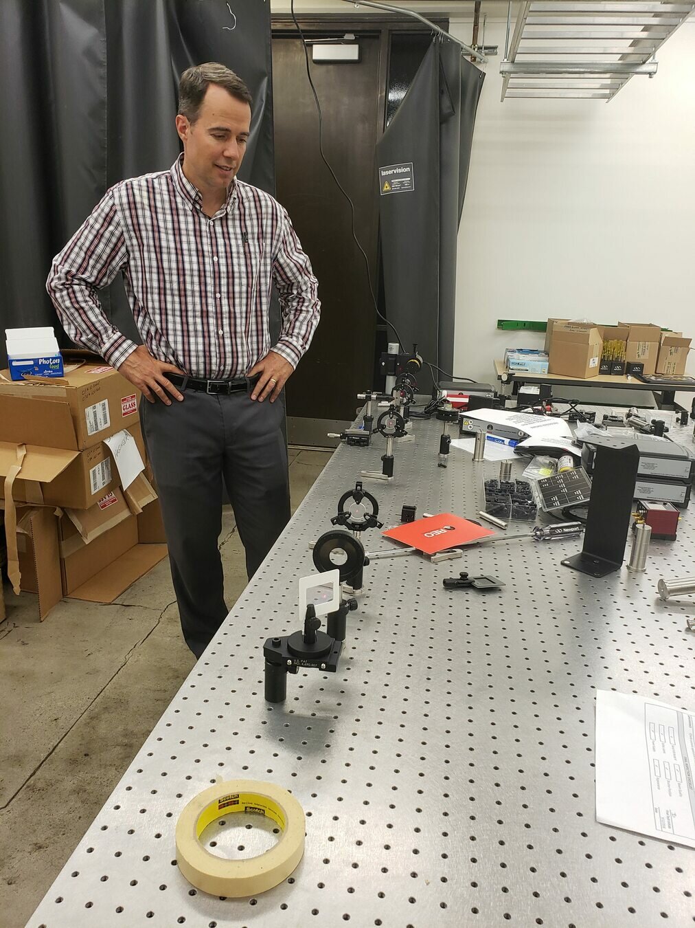
Optical Ventriloquism
Generating the standard superoscillation function in the lab is difficult.
But, all you need to shift the apparent source
of a light beam is wave interference that breaks the usual assumptions of geometric ray optics.
We used a single slit diffraction pattern.
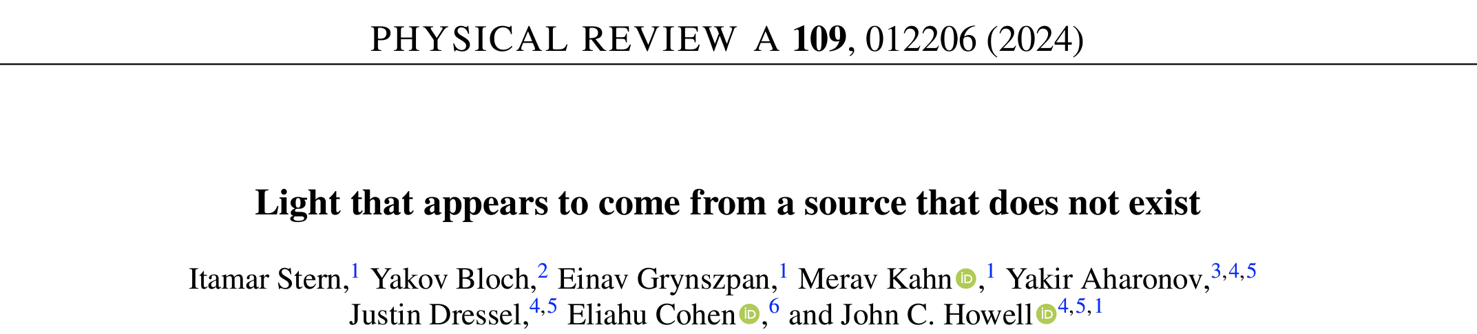
PRA 109, 012206 (2024)
Optical Ventriloquism
The key is to look at the local wave-vector \(\vec{k}\) at a particular location far from the slit.
This is done by seeing how the centroid shifts a short distance after a pinhole.
(This requires a high-resolution centroid measurement after the pinhole, like a knife-edge scan across a bucket detector.)
If you were at the pinhole and looked for the source, you would see it as coming from the direction of the local wave-vector.
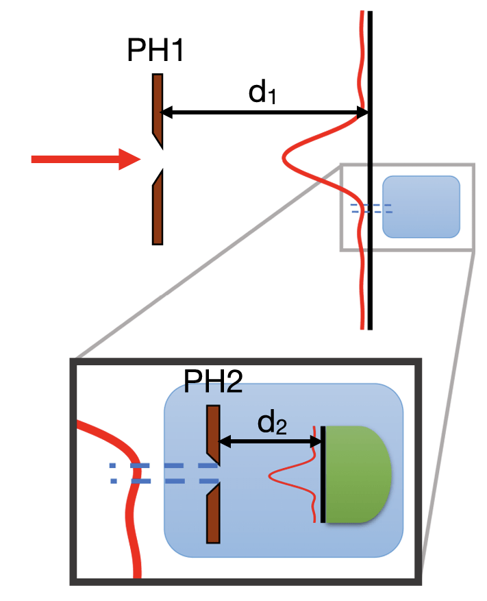
PRA 109, 012206 (2024)
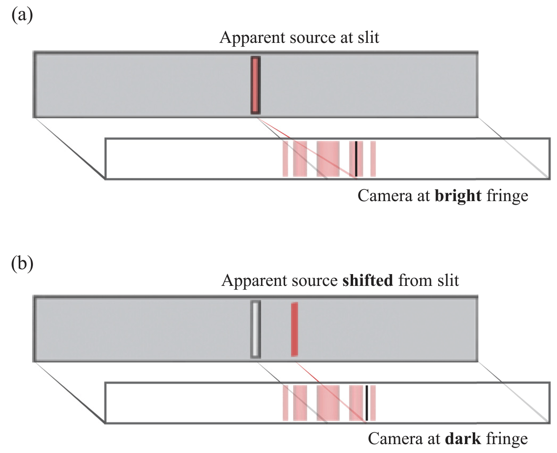
Optical Ventriloquism
In the bright fringes, the wave vector correctly comes from the slit location.
But near dark fringes, the wave vector rotates locally so \(k_x\approx 0\), so it looks like it
came from a different location!
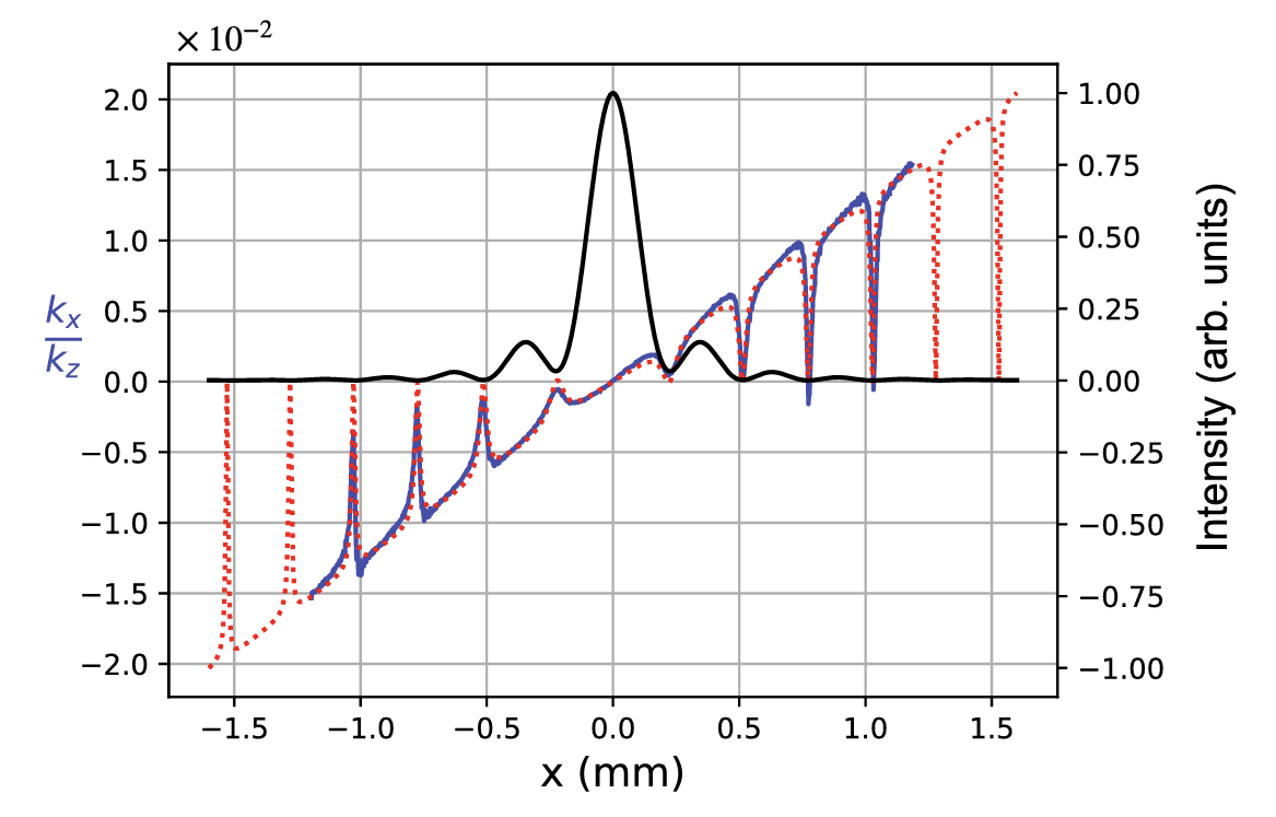
Blue: Experimental data for \(k_x/k_z\)
Red: Theoretical prediction for \(k_x/k_z\)
Black: Intensity profile at pinhole
PRA 109, 012206 (2024)
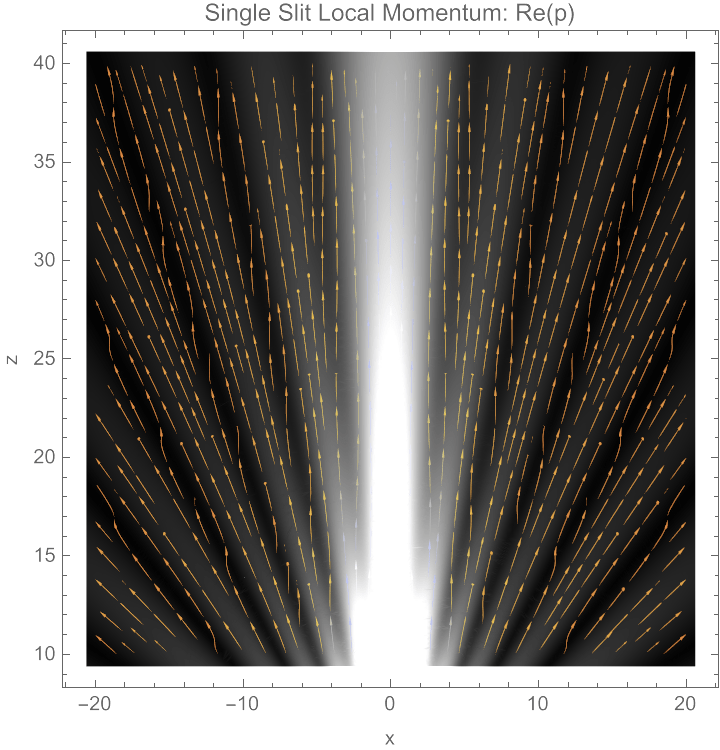
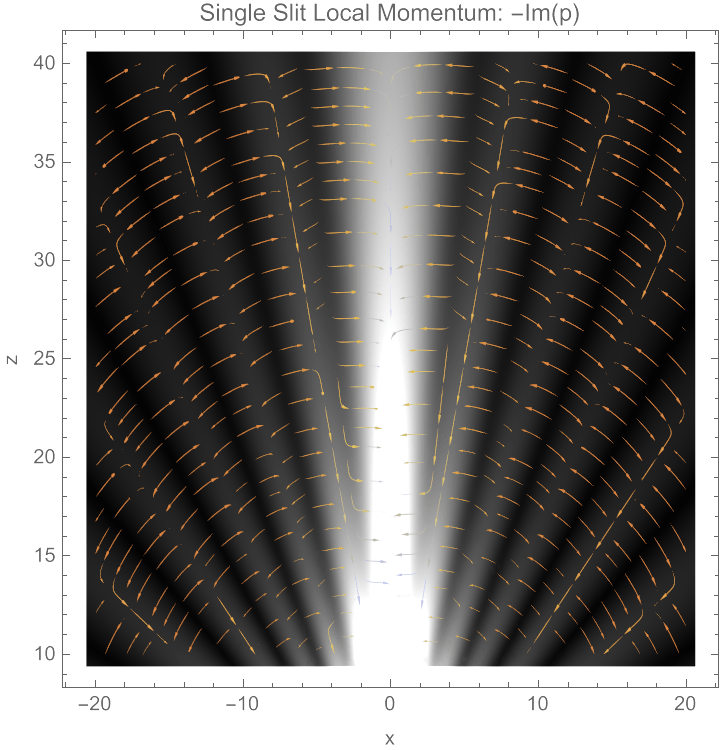
Single Slit Streamlines
PRA 109, 012206 (2024)
Single Slit Far-Field Slice
PRA 109, 012206 (2024)
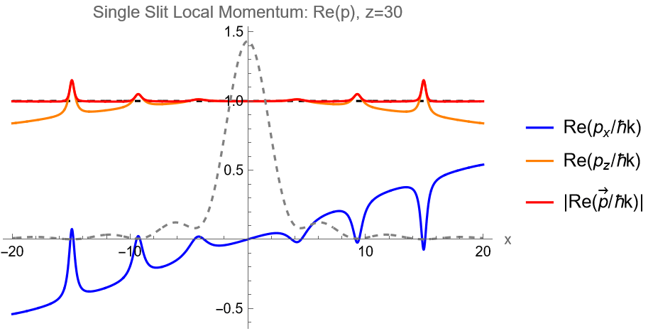

Superoscillations near interference zeroes
(\(|\vec{p}|\) exceeds \(\hbar k\) locally)
Same resonance-like structure where superoscillations occur
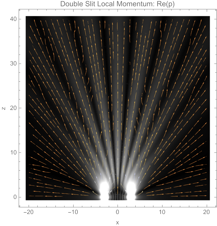
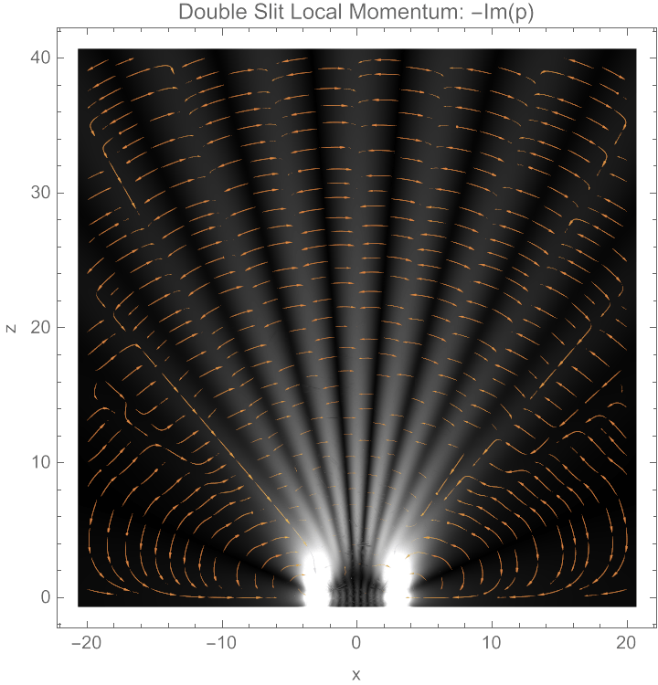
Double Slit Streamlines
PRA 109, 012206 (2024)
Double Slit Far-Field Slice
PRA 109, 012206 (2024)
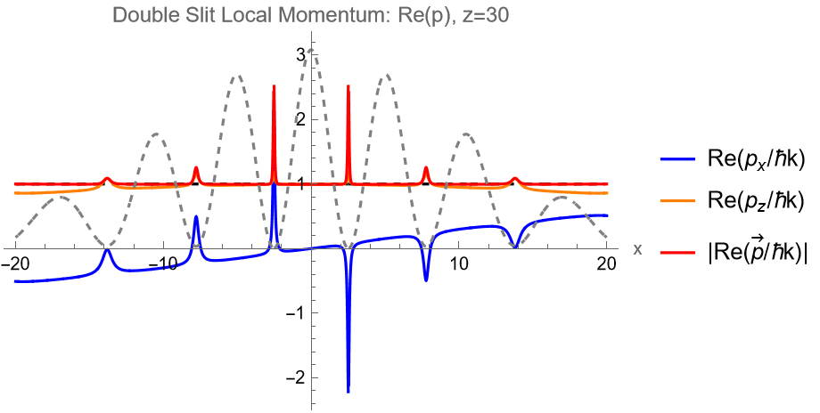
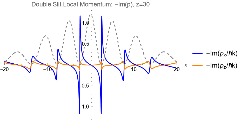
Superoscillations near interference zeroes
(\(|\vec{p}|\) exceeds \(\hbar k\) locally)
Same resonance-like structure where superoscillations occur
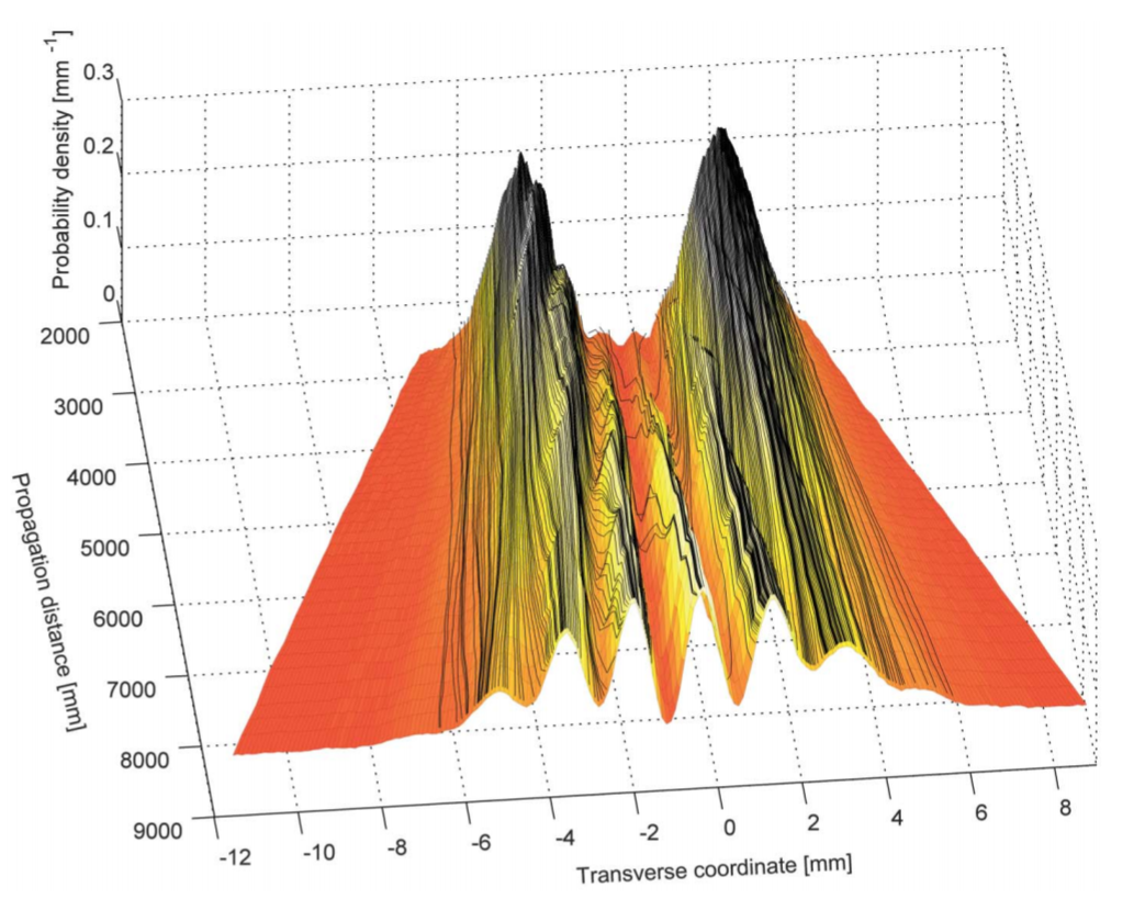
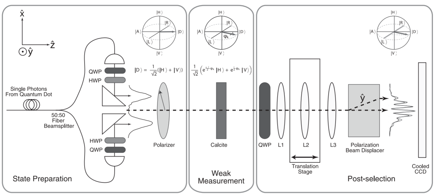
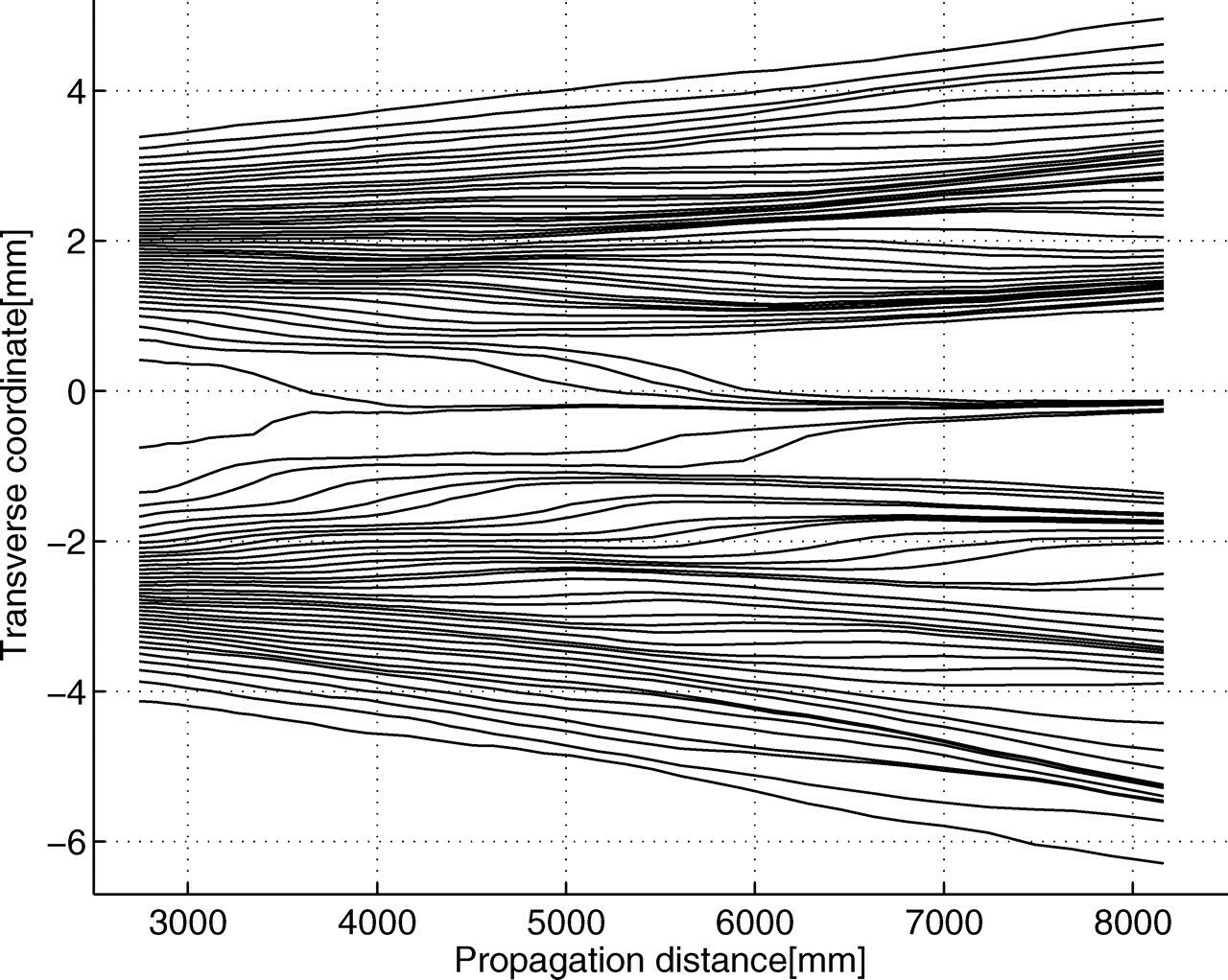
Experimental Double-Slit Streamlines
Local momentum weak measurements yield "averaged trajectories" for the mean momentum streamlines.
More complete streamlines measured by Steinberg group.
Kocsis et al., Science (2011)
Note: If the local momentum of the beam is rotating, there must be a local force.
There is no external force besides the beam itself, so the internal amplitude structure of the wave must be self-bending its own local momentum!
Local Energy-Momentum
Generalizing to local energy-momentum measured by a probe at spacetime point \((t,\vec{x})\):
\displaystyle \vec{p}(t,x) \equiv \frac{\langle \vec{x} | \hat{\vec{p}} | \psi(t) \rangle}{\langle \vec{x} | \psi(t) \rangle} = \frac{-i\hbar\vec{\nabla}\psi(t,\vec{x})}{\psi(t,\vec{x})} = \vec{\nabla} S(t,\vec{x})
\displaystyle \psi(t,\vec{x}) \equiv \langle \vec{x} | \psi(t) \rangle = \exp(iS(t,\vec{x})/\hbar)
Here \(S(t,\vec{x})\) is the (complex) eikonal for the (relativistic) wave-function \(\psi(t,\vec{x})\).
For a simple plane wave, the eikonal is linear with constant amplitude \(A\):
\displaystyle S(t,\vec{x}) \equiv (S_0 - i\hbar \ln A) + \hbar(\vec{k}\cdot\vec{x} - \omega t)
\displaystyle E(t,\vec{x}) \equiv \frac{\langle \vec{x} | \hat{E} | \psi(t) \rangle}{\langle \vec{x} | \psi(t) \rangle} = \frac{i\hbar\partial_t\psi(t,\vec{x})}{\psi(t,\vec{x})} = -\partial_t S(t,\vec{x})
\displaystyle \vec{p} = \vec{\nabla} S = \hbar \vec{k}, \quad E = -\partial_t S = \hbar\omega
Weak value prescription correctly reproduces both the Hamilton-Jacobi
definition of energy-momentum and the DeBroglie relations.
Wave Equation: Eikonals
Consider a wave equation:
\displaystyle \psi(t,\vec{x}) \equiv \exp(iS(t,\vec{x})/\hbar)
This is equivalent to the complex eikonal equation:
Assume \(\omega\) is real and constant in \(t\) (monochromatic). Split equations:
\begin{aligned}
\displaystyle \vec{p} &= \vec{\nabla} S = \hbar \vec{k} = \hbar (\vec{k}_r + i \vec{k}_i) \\
E &= -\partial_t S = \hbar\omega
\end{aligned}
\displaystyle \left[\frac{n^2}{c^2}\partial_t^2 - |\vec{\nabla}|^2\right]\psi(t,\vec{x}) = 0
\displaystyle (\partial_t S)^2 -i\hbar\partial_t(\partial_t S) = \frac{c^2}{n^2}[\vec{\nabla} S \cdot\vec{\nabla}S -i\hbar\vec{\nabla}\cdot(\vec{\nabla} S)]
\displaystyle \omega^2 +i\partial_t\omega = \frac{c^2}{n^2}[\vec{k}\cdot\vec{k} -i\vec{\nabla}\cdot\vec{k}]
\begin{aligned}
\displaystyle \omega &= \frac{c}{n}\sqrt{|\vec{k}_r|^2 - |\vec{k}_i|^2 + \vec{\nabla}\cdot\vec{k}_i} = \frac{c}{n}\sqrt{|\vec{k}_r|^2 - |\vec{\nabla}|^2|\psi|/|\psi|} \\
\vec{\nabla}\cdot\vec{k}_r &= 2\vec{k}_r\cdot \vec{k}_i
\end{aligned}
(Dispersion relation)
(Source relation)
Deviations from geometric optics caused by "Optical (Quantum) Potential"
Generalizing Geometric Optics
\begin{aligned}
\displaystyle \omega &= \frac{c}{n}\sqrt{|\vec{k}_r|^2 - |\vec{k}_i|^2 + \vec{\nabla}\cdot\vec{k}_i} = \frac{c}{n}\sqrt{|\vec{k}_r|^2 - |\vec{\nabla}|^2|\psi|/|\psi|} \\
\vec{\nabla}\cdot\vec{k}_r &= 2\vec{k}_r\cdot \vec{k}_i
\end{aligned}
Modified Ray Equations:
\begin{aligned}
\displaystyle \frac{d\vec{x}}{dt} &= \frac{\partial \omega}{\partial\vec{k}_r} = \frac{c^2}{n^2}\frac{\vec{k}_r}{\omega} \\
\frac{d\vec{k}_r}{dt} &= -\vec{\nabla}\omega = -\vec{\nabla}\left[-\frac{c^2}{n^2\omega}\frac{|\vec{\nabla}|^2|\psi|}{\psi}\right]
\end{aligned}
Optical self-bending caused by "Optical (Quantum) Potential"
Classical EM Field Momentum
Momentum weak value proportional to the local (orbital part of the time-averaged)
Poynting vector \(\vec{S}_O = \vec{E}^*\cdot(\vec{\nabla})\vec{E}\), scaled by the energy density \(W\).
This quantity exactly corresponds to the transferrable momentum
available locally via the spin-independent part of the stress-energy tensor of the field.
This momentum weak value weighted by the energy density correctly gives the local optical force felt by small probe particles with complex susceptibility \(\chi\):
Kocsis et al., Science (2011)
Bliokh et al. NJP (2013)
\displaystyle \text{Re}\,\mathbf{p}(\mathbf{r}) = \text{Re} \frac{\langle x | \hat{p} | \psi \rangle}{\langle x | \psi \rangle} = \frac{\omega}{c^2} \frac{S_o(\textbf{r})}{W(\textbf{r})}
Light isn't a massive fermion, so why does this prescription work in the EM case?
\begin{aligned}
\displaystyle \vec{F} &= \frac{1}{2}\left[\text{Re}\chi\,\text{Re}\vec{E}^*\cdot(\vec{\nabla})\vec{E} - \text{Im}\chi\,\text{Im}\vec{E}^*\cdot(\vec{\nabla})\vec{E}\right] = \vec{F}_{\rm gradient} + \vec{F}_{\rm scatter}
\end{aligned}
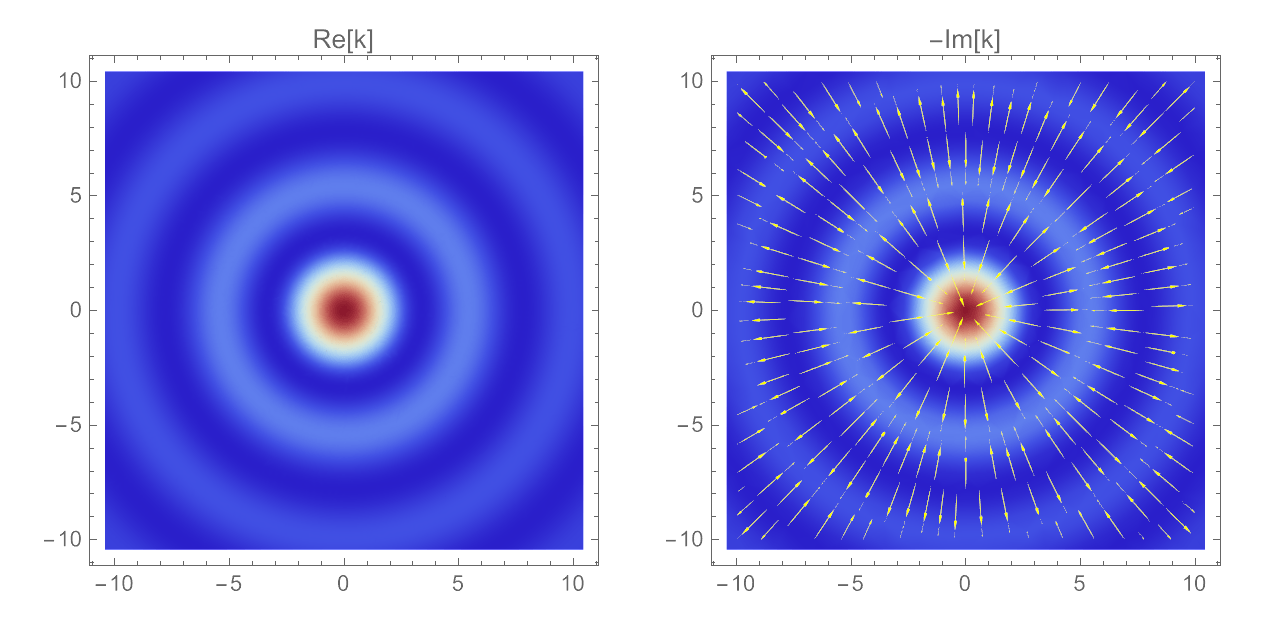
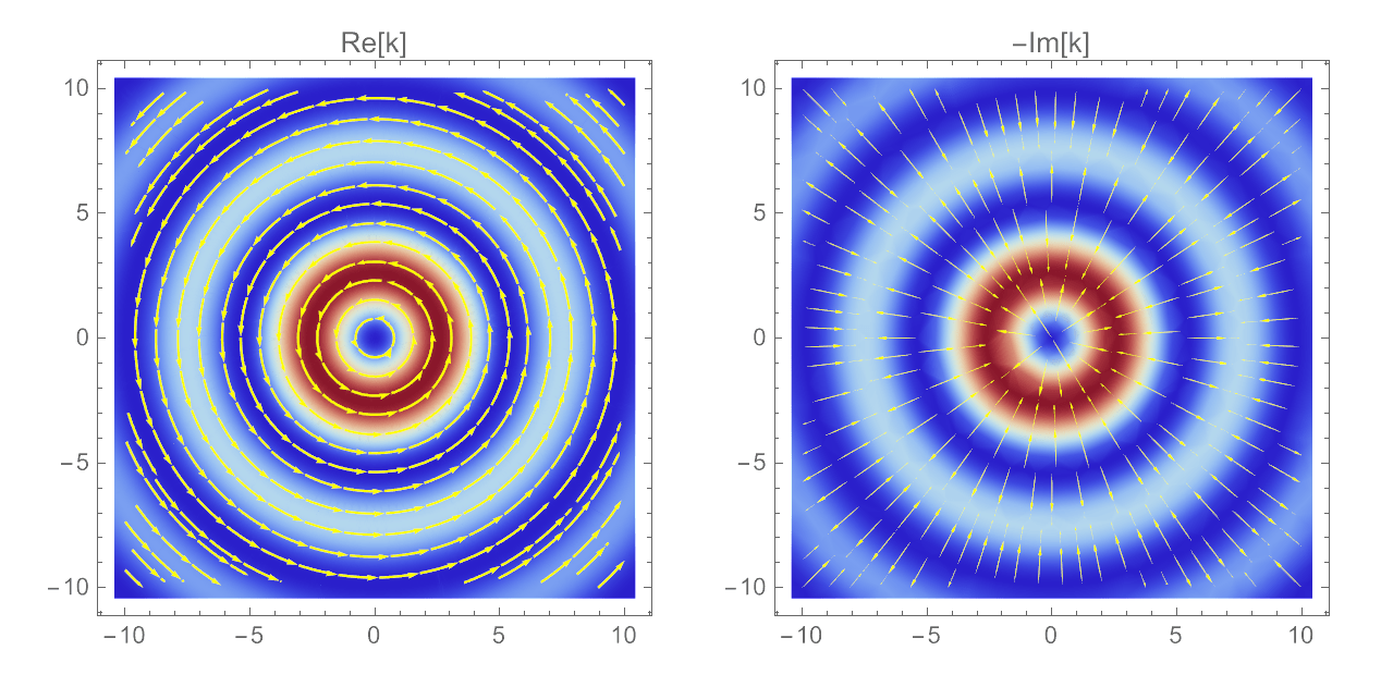
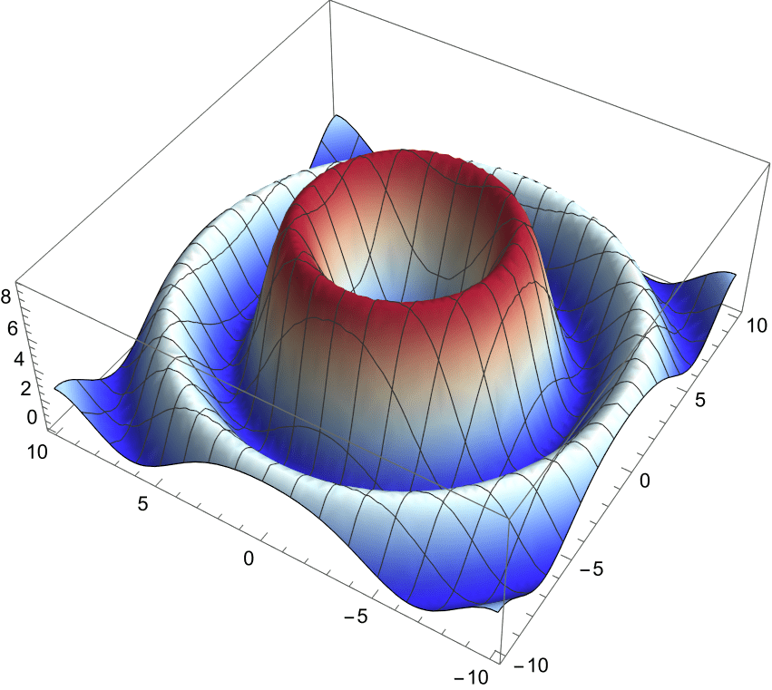
Illustrated Example: Bessel beams
Both real and imaginary parts of this local momentum average also describe physical properties of classical "vortex beams" like Bessel beams.
\displaystyle \mathbf{p}_w(\mathbf{r}) = \frac{\langle x | \hat{p} | \psi \rangle}{\langle x | \psi \rangle}
The real part of the momentum weak value appears as the circulating local orbital momentum for higher-order Bessel beams that can be transferred to probe particles by pushing them around in circular orbits.
The imaginary part is also meaningful and directed radially to confine the optical intensity into concentric rings.
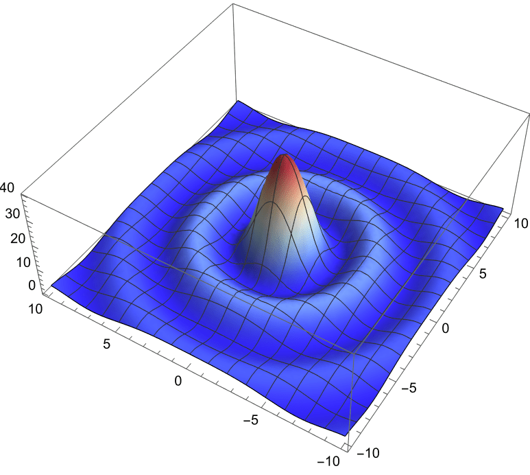
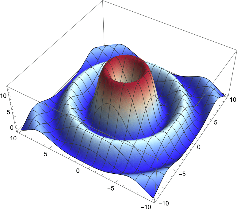
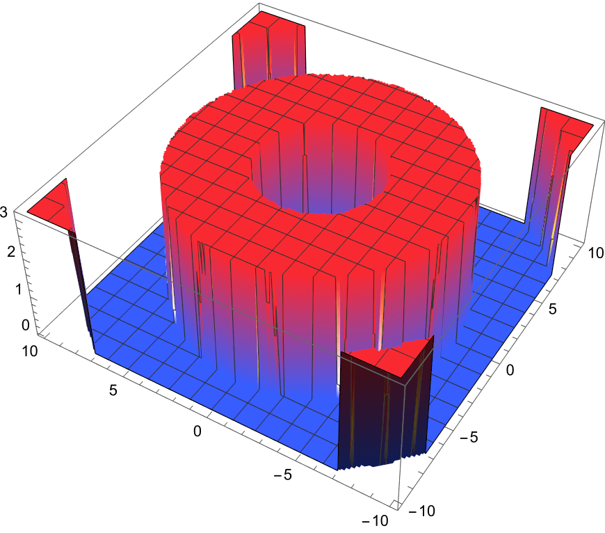
0th-Order Bessel Beam
The basic Bessel beam has zero orbital angular momentum.
The phase fronts are parallel to the transverse plane.
The local \(\vec{k}(\vec{r})\) are directed only along
the propagation axis \(z\), so \(k_x = k_y = 0\).
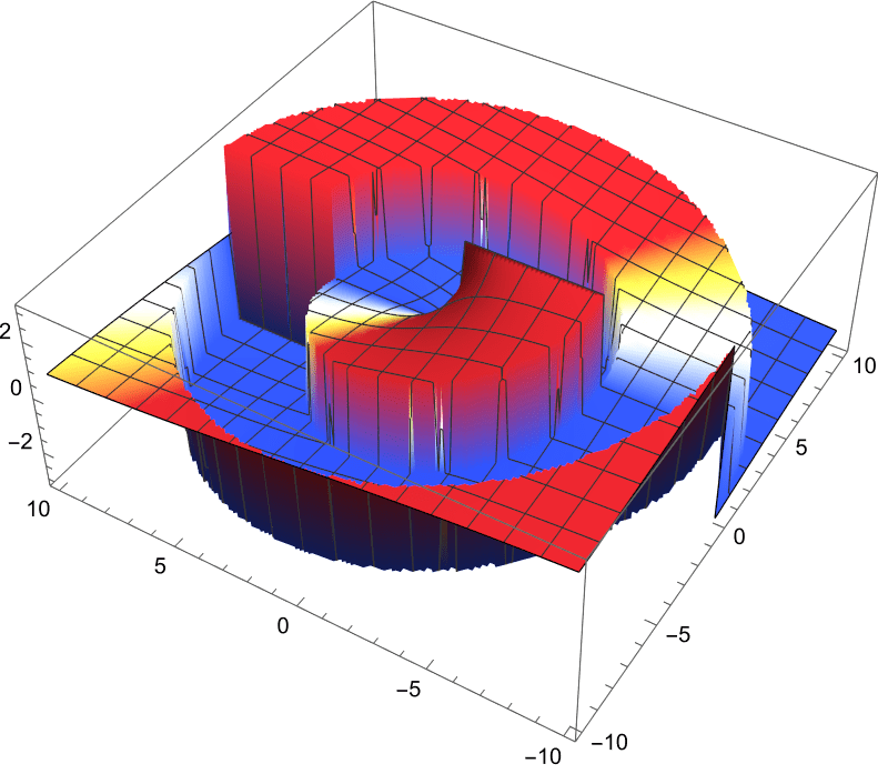
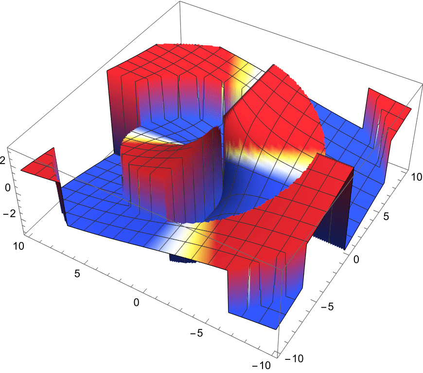
1st-Order Bessel Beam
The 1st-order Bessel beam has non-zero orbital angular momentum.
The phase fronts are helices so are angled from the transverse plane.
The local \(\vec{k}(\vec{r})\) are circulating in the transverse \(x\)-\(y\) plane,
exactly as you would expect for orbital angular momentum.
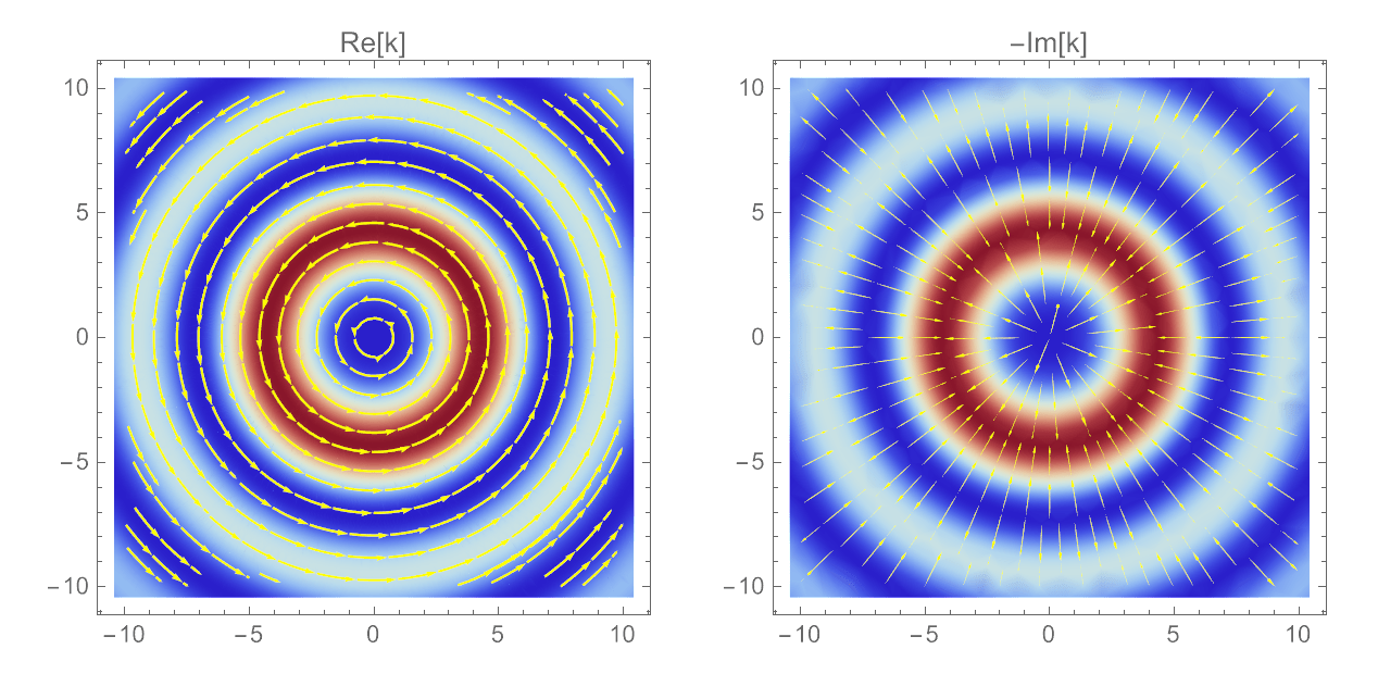
2nd-Order Bessel Beam
The 2nd-order Bessel beam has larger orbital angular momentum.
The phase fronts are steeper helices so orbit faster.
The local \(\vec{k}(\vec{r})\) also circulate faster in the transverse \(x\)-\(y\) plane,
with a larger radius as expected.
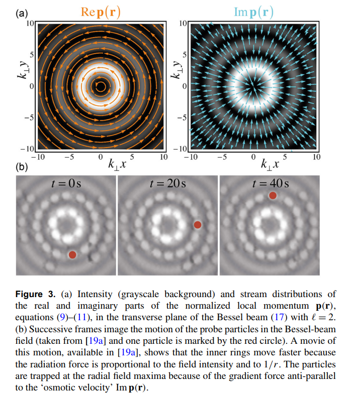
Experimental Bessel Beam
Bliokh et al., NJP (2013)
Experiments placing small probe particles in a 2nd-order Bessel beam show that the particles begin orbiting within the circular rings and remain confined to the bright regions.
\displaystyle \mathbf{p}_w(\mathbf{r}) = \frac{\langle x | \hat{p} | \psi \rangle}{\langle x | \psi \rangle}
The real part of the momentum weak value is transferred to probe particles as the gradient force and pushes them around in circular orbits.
The imaginary part is directed radially and confines the optical intensity into concentric rings, similarly redirecting absorptive probe particles as the scattering force to orbit only within the optical rings.
Thank You!
Optical Ventriloquism and Local Streamlines
By Justin Dressel
Optical Ventriloquism and Local Streamlines
Invited talk for the Superoscillations Conference, 2024/06/15


