Delayed Choice Qubit
Lorentz Transformations
Justin Dressel
Institute for Quantum Studies
Schmid College of Science and Technology


Outline:
-
Qubits have a 4D "spacetime" representation
- Pauli spin basis is a 3D Clifford algebra
- Measurements rotate hyperbolically into 4D
-
Continuous measurements behave like (stochastic) Lorentz transformations
-
Circuit QED implementations are naturally "delayed choice" continuous measurements
- Long after a probing microwave field interacts with the qubit, the choice of amplified quadrature selects which type of Lorentz transformation was performed
Example: Monitored Rabi Oscillations
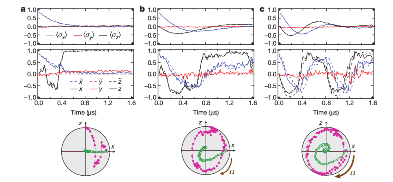
A monitored quantum system (here a transmon qubit) has both smooth unitary dynamics and random measurement backaction
UCB, Nature 511, 570 (2014)
The composite dynamics has interesting theoretical structure
Qubits are 4-dimensional
- Qubits (e.g., spin-1/2) are 2-level quantum systems
- But, qubit state space is generally 4-dimensional
|\psi\rangle = \alpha |0\rangle + \beta |1\rangle
\hat{\rho} = \frac{1}{2}\left(p \hat{1} + x \hat{\sigma}_1 + y \hat{\sigma}_2 + z \hat{\sigma}_3\right)
State norm
(preparation success probability)
(max radius of Bloch sphere)
(Conditional) Expectation values
(Bloch sphere coordinates)
\hat{\sigma}_1 = |0\rangle\langle 1| + |1\rangle\langle 0|
\hat{\sigma}_2 = -i(|0\rangle\langle 1| - |1\rangle\langle 0|)
\hat{\sigma}_3 = |1\rangle\langle 1| - |0\rangle\langle 0|
x^2 + y^2 + z^2 \equiv R^2 \leq p^2
\hat{1} = |1\rangle\langle 1| + |0\rangle\langle 0|
Operator basis: Pauli operators
Orthonormal under operator inner product:
\hat{A}\cdot\hat{B} \equiv \frac{1}{2}\text{Tr}\left[\frac{\hat{A}\hat{B}+\hat{B}\hat{A}}{2}\right]
Pauli Operators form a 3D Clifford Algebra (for spin)
- The Clifford algebra of 3-space has 8 elements
- The 4 "grades" of the algebra correspond geometrically to oriented subspaces of differing dimensions
\hat{\sigma}_x\hat{\sigma}_y\hat{\sigma}_z
\hat{\sigma}_y\hat{\sigma}_z \quad \hat{\sigma}_z\hat{\sigma}_x \quad \hat{\sigma}_x\hat{\sigma}_y
\hat{\sigma}_x \quad \hat{\sigma}_y \quad \hat{\sigma}_z
\hat{1}
Geometric meaning:
Grade
0
1
2
3
Point
Line Segment
Plane Segment
Volume Segment
Matrix Representation of 3D Clifford Algebra
- Simplification:
i\hat{1}
i\hat{\sigma}_x \quad i\hat{\sigma}_y \quad i\hat{\sigma}_z
\hat{\sigma}_x \quad \hat{\sigma}_y \quad \hat{\sigma}_z
\hat{1}
Geometric meaning:
Grade
0
1
2
3
Point
Line Segment
Plane Segment
Volume Segment
\hat{\sigma}_x\hat{\sigma}_y\hat{\sigma}_z = i\hat{1}
(Representation-independent definition of "imaginary unit")
Dot and Wedge Products
The usual Pauli operators are a faithful matrix representation, so the matrix product is precisely the Clifford product
\hat{A}\hat{B} = \frac{\hat{A}\hat{B}+\hat{B}\hat{A}}{2} + \frac{\hat{A}\hat{B}-\hat{B}\hat{A}}{2}
Symmetric part is dot product
Antisymmetric (noncommutative) part is wedge product
\frac{\hat{A}\hat{B}+\hat{B}\hat{A}}{2} = (\hat{A}\cdot\hat{B})\hat{1}
\frac{\hat{A}\hat{B}-\hat{B}\hat{A}}{2} = \hat{A}\wedge\hat{B}
Unit operator is an artifact of the matrix representation
\langle \hat{A} \rangle_0 \equiv \frac{1}{2}\text{Tr}[\hat{A}]
Scalar projection removes representation:
\star \hat{A} \equiv -i\hat{A}
Hodge Star operation flips grade k to (3-k):
Cross Product is closed for grade 1 (vectors):
\hat{\sigma}_i\times\hat{\sigma}_j \equiv -i(\hat{\sigma}_i\wedge\hat{\sigma}_j) = \epsilon_{ijk}\hat{\sigma}_k
(Same "noncommutativity" in classical mechanics)
Why do we care?
For a physical spin, we expect rotations in 3D space to be relevant.
Identifying the implicit Clifford algebra makes geometry explicit.
\vec{s} \equiv \sum_j s_j\,\hat{\sigma}_j
A spin vector can be interpreted as a true vector in 3D space with this mapping.
\dot{\vec{s}} = \vec{\Omega}\times\vec{s} = -i(\vec{\Omega}\wedge\vec{s}) = \frac{-i}{2}\left[\vec{\Omega}\vec{s}-\vec{s}\vec{\Omega}\right] \equiv \frac{-i}{2}[\vec{\Omega},\vec{s}]
Classical spin precession becomes obviously the same as the commutator evolution generated by a Hamiltonian operator:
\hat{\rho} = \frac{1}{2}[p\hat{1} + \vec{s}]
\text{Tr}[\hat{\rho}\vec{\ell}] = \langle(p\hat{1} + \vec{s})\vec{\ell}\rangle_0 = \vec{s}\cdot\vec{\ell}
The physical correspondence of the state to spin orientations becomes transparent:
What about Measurement?
- The Clifford algebra of 3D space works for Hamiltonian evolution, since the norm of the state never changes
- Measurement changes the state norm
- We either need nonlinear evolution (renormalization), or we need to consider the 4th state component.
\hat{\rho} \mapsto |0\rangle\langle 0|\hat{\rho}|0\rangle\langle 0| = \frac{p-z}{2}|0\rangle\langle 0| = \frac{p-z}{4}(\hat{1}-\hat{\sigma}_z)
Example: ground-state projection
Equivalent to:
p \mapsto (p-z)/2
z \mapsto (z-p)/2
The state norm and spin components become
intertwined by measurement (before renormalization)
Gaussian Measurements
- Weak measurements provide much more intuition about how to handle the change of the state norm
Example:
\hat{\rho} \mapsto \hat{M}_r\hat{\rho}\hat{M}_r^\dagger = C^2(r)[\frac{p-z}{2}e^{-r/V}|0\rangle\langle 0| + \frac{p+z}{2}e^{r/V}|1\rangle\langle 1| + \frac{x}{2}\hat{\sigma}_x + \frac{y}{2}\hat{\sigma}_y]
Hyperbolic rotation of state components in p-z plane by "rapidity" angle r/V
\hat{M}_r = \frac{\exp[-(r-\hat{\sigma}_z)^2/4V]}{(2\pi V)^{1/4}} = C(r)\,e^{r\hat{\sigma}_z/2V}
P(r) = \frac{\text{Tr}[\hat{M}^\dagger_r\hat{M}_r\hat{\rho}]}{\text{Tr}[\hat{\rho}]} = P_{z=1}\frac{\exp(-(r-1)^2/2V)}{\sqrt{2\pi V}} + P_{z=-1}\frac{\exp(-(r+1)^2/2V)}{\sqrt{2\pi V}}
Gaussian pointer r of variance V centered on z eigenvalues +/- 1
C^2(r) = \frac{\exp(-(r^2+1)/2V)}{\sqrt{2\pi V}}
p \mapsto p\cosh(r/V)+z\sinh(r/V)\qquad z\mapsto z\cosh(r/V)+p\sinh(r/V)
State update:
Measurement (Kraus) operator:
prefactor cancels in state renormalization: neglect (This abandons probabilistic interpretation)
Continuous Measurements
- Every time step dt is a Gaussian measurement with variance:
Instantaneous "rapidity" angle:
\hat{M}_r = \frac{\exp[-dt(r-\hat{\sigma}_z)^2/4\tau]}{(2\pi \tau/dt)^{1/4}} = C(r)\,e^{dt\,r\hat{\sigma}_z/2\tau}
C^2(r) = \frac{\exp(-dt(r^2+1)/2\tau)}{\sqrt{2\pi \tau/dt}}
p \mapsto p\cosh(dt\,r/\tau)+z\sinh(dt\,r/\tau)\qquad z\mapsto z\cosh(dt\,r/\tau)+p\sinh(dt\,r/\tau)
State update:
Measurement (Kraus) operator:
V = \tau/dt
dt\,r/\tau
\text{In the limit }dt\to 0\text{ the measurement becomes continuous.}
\text{Purity-preserving, Markovian measurements fully characterized by timescale }\tau
\text{Readout }r\text{ then is white noise around the moving mean }\langle\hat{\sigma}_z\rangle
Purity-preserving measurement preserves invariant interval:
p^2 - (x^2 + y^2 + z^2) \geq 0
4D Clifford Algebra
Rotations in planes involving the state norm are hyperbolic.
Rotations in planes not involving the state norm are elliptic.
This is equivalent to the structure of spacetime.
Note: it is simple to "upgrade" the qubit representation to this 4D "spacetime"
3D Clifford algebra is a subalgebra of the 4D Clifford algebra of spacetime
Removing matrix representation changes no physics, but clarifies correspondence
\gamma_0,\,\gamma_1,\,\gamma_2,\,\gamma_3
\sigma_1,\,\sigma_2,\,\sigma_3\quad\mapsto
Euclidean 3D
Minkowski 4D (+,-,-,-)
\sigma_1^2 = \sigma_2^2 = \sigma_3^2 = 1
\gamma_0^2 = 1, \; \gamma_1^2 = \gamma_2^2 = \gamma_3^2 = -1
\sigma_1 \equiv \gamma_1\gamma_0 \quad \sigma_2 \equiv \gamma_2\gamma_0 \quad \sigma_3 \equiv \gamma_3\gamma_0
Apparent 3D vectors are timelike planes in 4D
Could represent 4D basis as Dirac "gamma matrices" if desired
(note vague connection to relativistic spin 1/2)
4D Clifford Algebra
- Simplification:
i
\sigma_1 \quad \sigma_2 \quad \sigma_3 \quad | \quad i\sigma_1 \quad i\sigma_2 \quad i\sigma_3
\gamma_0 \quad | \quad \gamma_1 \quad \gamma_2 \quad \gamma_3
1
Grade
0
1
2
3
i \equiv \sigma_1\sigma_2\sigma_3 = \gamma_0\gamma_1\gamma_2\gamma_3
(Representation-independent definition of "imaginary unit")
(but, commutes with even grade, anti-commutes with odd grade)
4
i\gamma_0 \quad | \quad i\gamma_1 \quad i\gamma_2 \quad i\gamma_3
2^4 = 16\;\text{elements}
Relative 3D space embedded as even-graded subspace
Planes (of rotation):
3 hyperbolic | 3 elliptic
\hat{\rho} = \frac{1}{2}(p\hat{1} + x\hat{\sigma}_1 + y\hat{\sigma}_2 + z\hat{\sigma}_3) \mapsto \rho \equiv p + x\sigma_1 + y\sigma_2 + z\sigma_3
\rho = (p\gamma_0 + x\gamma_1 + y\gamma_2 + z\gamma_3)\gamma_0 = \rho\!\!\!/ \gamma_0
4D "Minkowski" Qubit
Drop 2D matrix representation, preserving physics in Clifford algebra:
Reinterpret algebra as embedded in 4D "spacetime":
Proper 4-vector
Proper time direction (of agent)
(defines relative space for rotations)
Rotations are then obvious spinor transformations of a proper 4-vector:
e^{dt(r/2\tau)(\sigma_3)}\rho e^{dt(r/2\tau)(\sigma_3)} = e^{dt(r/2\tau)(\sigma_3)}\rho\!\!\!/ e^{-dt(r/2\tau)(\sigma_3)}\gamma_0
e^{dt(\Omega/2)({\star}\sigma_1)}\rho e^{-dt(\Omega/2)({\star}\sigma_1)} = e^{dt(\Omega/2)({\star}\sigma_1)}\rho\!\!\!/ e^{-dt(\Omega/2)({\star}\sigma_1)}\gamma_0
Hamiltonian:
Measurement:
\text{Elliptic rotation in spatial (spin) plane }{\star}\sigma_1 = -i\sigma_1 = \gamma_2\gamma_3\text{ with spin axis }\sigma_1
\text{Hyperbolic rotation (boost) in temporal (measurement) plane }\sigma_3 = \gamma_3\gamma_0
Recall: p not probability after rotation
Classical spin "hidden variable" model
4D Matrix Representation
- While a spinor representation of 4D rotations is efficient, a 4x4 real matrix representation is also computationally useful
\rho\!\!\!/ \mapsto \begin{bmatrix}p \\ x \\ y \\ z\end{bmatrix}
e^{dt\,F/2}\rho\!\!\!/ e^{-dt\,F/2} \mapsto \exp\left(dt\begin{bmatrix}0 & r_x/\tau & r_y/\tau & r_z/\tau \\ r_x/\tau & 0 & -\Omega_z & \Omega_y \\ r_y/\tau & \Omega_z & 0 & -\Omega_x \\ r_z/\tau & -\Omega_y & \Omega_x & 0\end{bmatrix}\right)\begin{bmatrix}p \\ x \\ y \\ z\end{bmatrix}
F = E + i B
E = (r_x/\tau)\sigma_1 + (r_y/\tau)\sigma_2 + (r_z/\tau)\sigma_3
iB = (\Omega_x){\star}\sigma_1 + (\Omega_y){\star}\sigma_2 + (\Omega_z){\star}\sigma_3
Effective "electric field" polarizes spin
Effective "magnetic field" rotates spin
Lorentz rotation generator equivalent to "electromagnetic field tensor"
Describes continuous monitoring of all three qubit measurement axes:
easily modified to add experimental inefficiencies (T1, T2, eta, etc.)
arXiv:1606.01407
Superconducting Qubit (3D Transmon)
"Qubit" is lowest two energy levels of a nonlinear oscillator
Not spin-1/2, but formalism still useful.
Yale, PRL 107, 240501 (2011)
Continuous Monitoring with Microwaves
Gaussian measurement per dt
Distinguishable qubit states
UCB, Nature 502, 211 (2013)
Phase-sensitive amplifier (LJPA) squeezes field along information-carrying quadrature
\text{Hamiltonian: }H_I = \chi\,\sigma_z\,a^\dagger a
Delayed Choice Rotations!
UCB, Nature 502, 211 (2013)
Note the temporal progression:
- Field interacts with qubit in cavity
- Field leaks from cavity (unsqueezed)
- Field propagates away for a delay
- Amplifier phase chooses squeezed quadrature
- Homodyne measures squeezed quadrature
F = e^{i\phi}(r/\tau)\sigma_3
Phase of squeezing axis chosen long after field escapes cavity: type of qubit Lorentz rotation depends on this phase!
Causality still Preserved
Same ensemble-averaged (Lindblad) dynamics must occur regardless of (later) choice of measurement (and collected information)
However, the physical story told by the observed readout will be very different
Korotkov, arXiv:1111.4016 (2011)
Fluctuations vs. Collapse
UCB, Nature 502, 211 (2013)
Story #1:
The squeezing eliminates distinguishability of qubit states, but amplifies the intrinsic uncertainty of the cavity field photon number.
The fluctuating photon number made the qubit energy fluctuate, creating random phase drifts that dephase the qubit in the ensemble average (purely elliptic rotations).
Story #2:
The squeezing suppresses the intrinsic photon number uncertainty, but amplifies the field separation between distinct qubit states..
The cavity photon number does not fluctuate. Instead, continuous weak monitoring of z creates partial collapses that decohere the qubit in the ensemble average (purely hyperbolic rotations).
The later choice of squeezing axis completely changes the physical picture.
Conclusions
- Two-level systems undergoing Gaussian continuous measurement have a natural mapping to stochastic Lorentz transformations of a 4-vector
- Circuit QED measurements have a naturally delayed choice for which Lorentz transformations have occurred
Thank you!
Delayed Choice Lorentz Rotations
By Justin Dressel
Delayed Choice Lorentz Rotations
An analysis of qubit evolution in terms of Lorentz transformations.


