What does a continuously monitored qubit readout really show?
Luis Pedro García-Pintos
Justin Dressel
APS March Meeting 2017

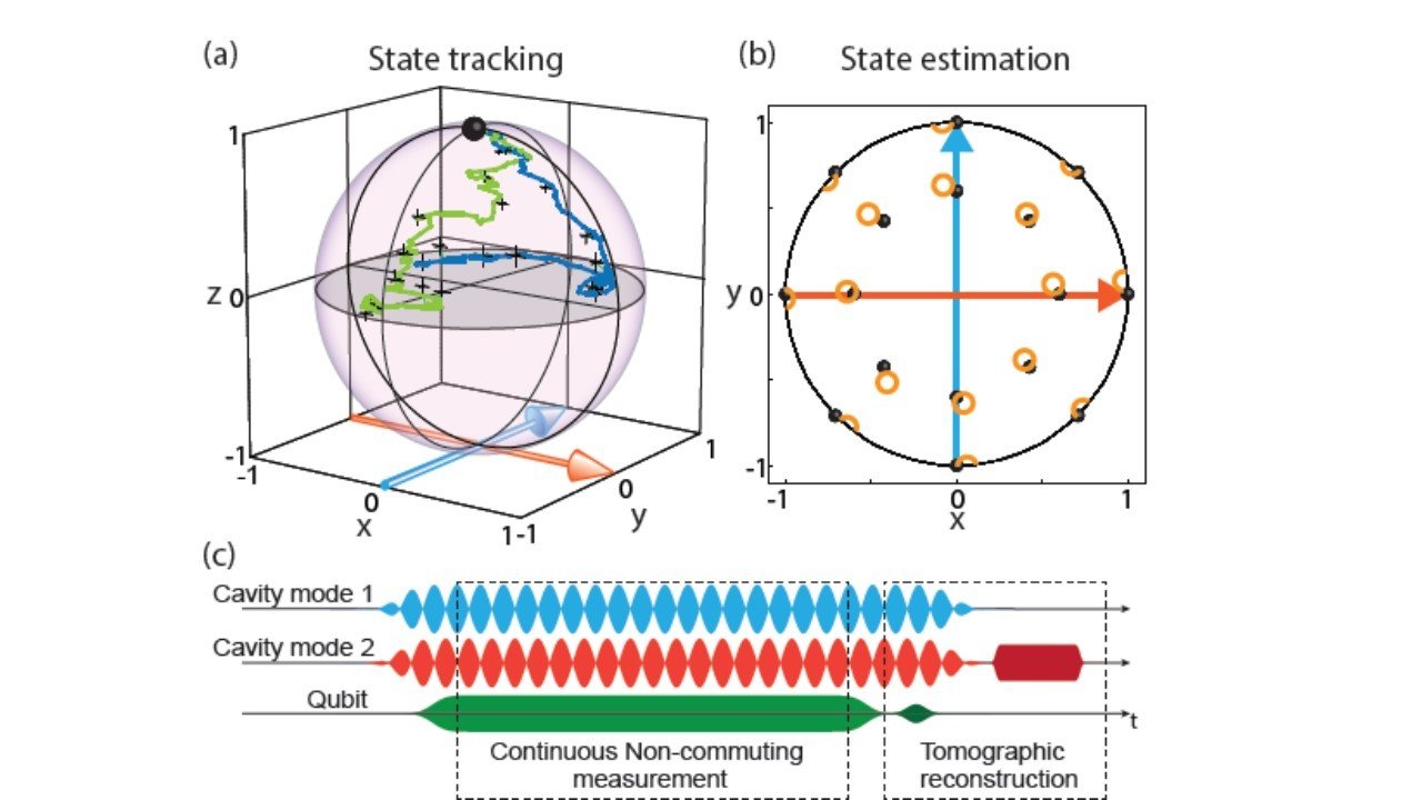
How do we know whether individual quantum state trajectories that we reconstruct from experimental data are correct, using the readout alone?
Current approach:
Perform a random tomographic pulse at the end of each data run
Spot check subensembles of data to verify tomography of final state
Motivation
Murch et al., Nature 502, 211 (2013)
Hacohen-Gourgy et al., Nature 538, 491 (2016)
If the collected stochastic signal noisily tracks an observable of the qubit, can we filter the signal to estimate that observable trajectory independently?
Idea: Filter the Readout
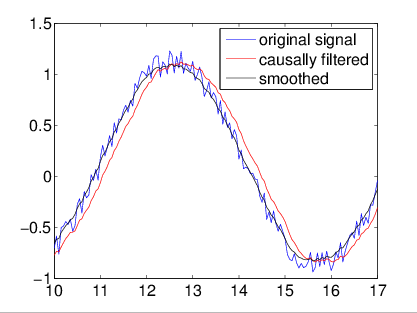
Classical signals can remove Gaussian noise either:
1) Causally (no future signal), with a filter (e.g. Weiner, Kalman)
2) Non-causally (using future signal), with a smoother
For already collected data, smoothers work best
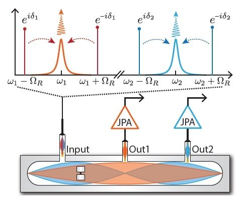
r(t) = z(t) + \sqrt{\tau}\,\xi(t)
Monitored qubit Z operator:
causally generated readout
Signal
Observ. Exp. Value
Gaussian Noise
Structure of collected qubit signal seems amenable to such a filtering technique
Filter independent of trajectory model
z(t) = \mathrm{Tr}[Z\,\rho_{\vec{r}_{\mathrm{past}}}]
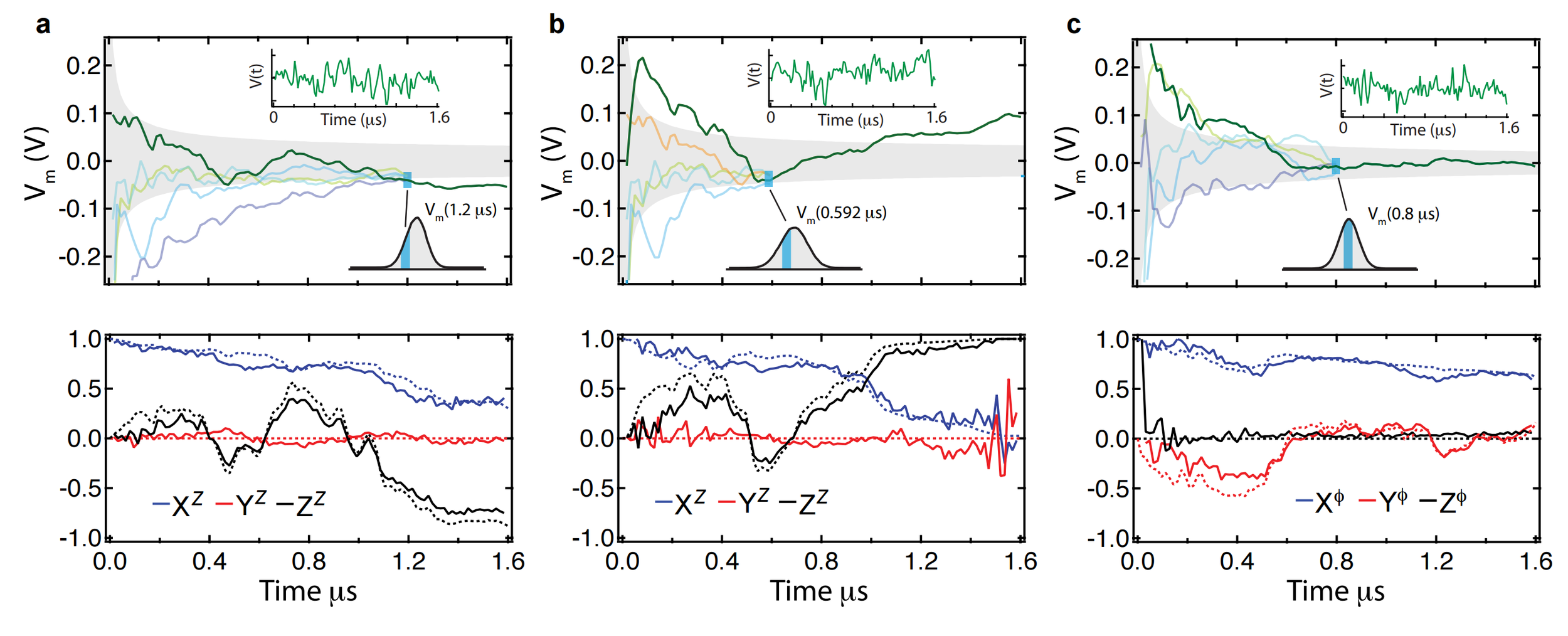
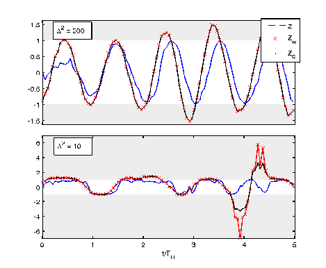
Evidence : Qubit Z
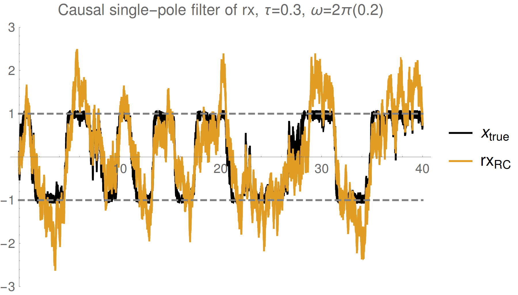
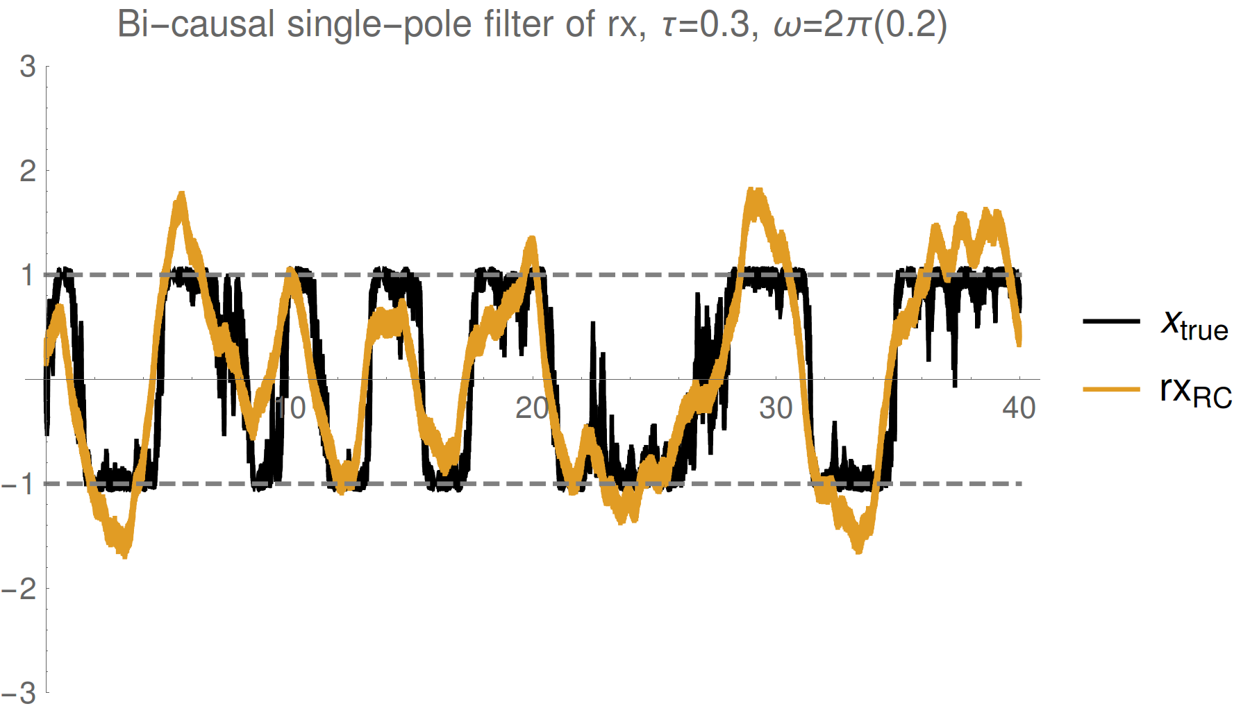
Simple single pole filter
Simple single pole smoother
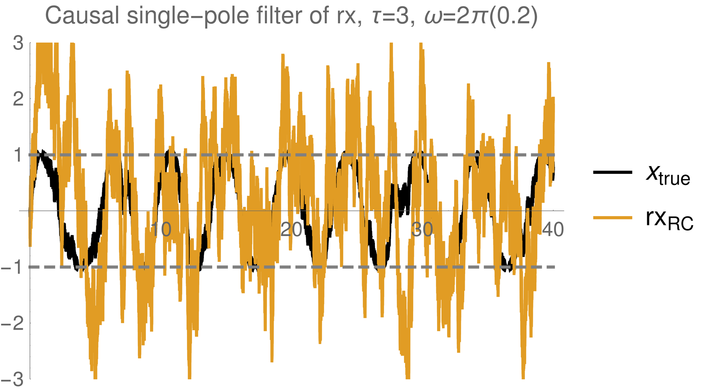
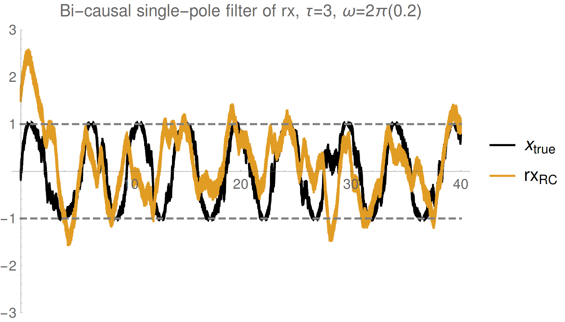
Strong (Zeno) regime: tracking jumps
Weak regime: tracking noisy Rabi oscillations
Trend : stronger measurements yield more information
--> better fidelity, but more perturbed evolution
Reasonable tracking
Noise harder to remove
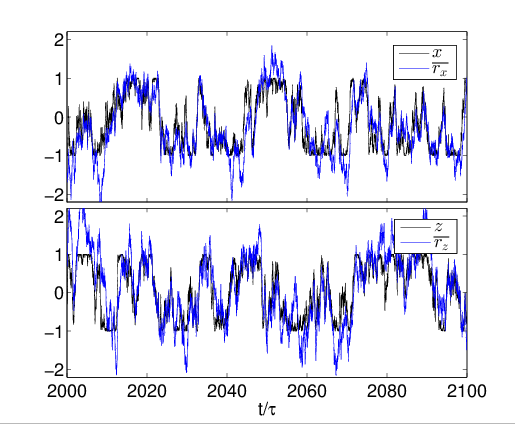
Evidence: Qubit X + Z
Simple single pole filter
Simultaneous (here X+Z) measurements work well
(with stronger measurements)
One can track multiple observables simultaneously for a single trajectory with reasonable (~90%) fidelity, without a master equation
Filtering idea works, but fidelity is limited. What is the theoretical limit?
see also Ruskov et al. PRL 105 100506 (2010): >90% state fidelity with 3 axis monitoring + filtering
Hacohen-Gourgy et al., Nature 538, 491 (2016)
Consider a single collected readout r(t), but omit one point at t=t1.
What distribution P[r(t1)] describes the likelihood of the omitted point?
Readout Distribution
P(r\, |\, \vec{r}_{\mathrm{past}},\, \vec{r}_{\mathrm{future}}) = \frac{P(r,\, \vec{r}_{\mathrm{future}}\,|\,\vec{r}_{\mathrm{past}})}{\sum_r P(r,\, \vec{r}_{\mathrm{future}}\,|\,\vec{r}_{\mathrm{past}})} \approx \frac{\exp\left[-\frac{dt}{2\tau}(r-z_s)^2\right]}{\sqrt{2\pi\tau/dt}}
Discretize time into bins of size dt - assume Markovian Gaussian measurements:
We recover approximate Gaussian noise, as expected:
r(t) = z_s(t) + \sqrt{\tau}\,\xi(t)
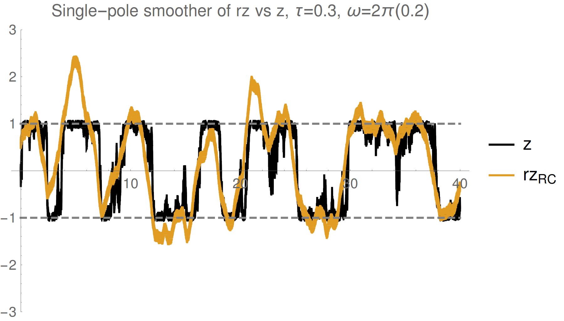
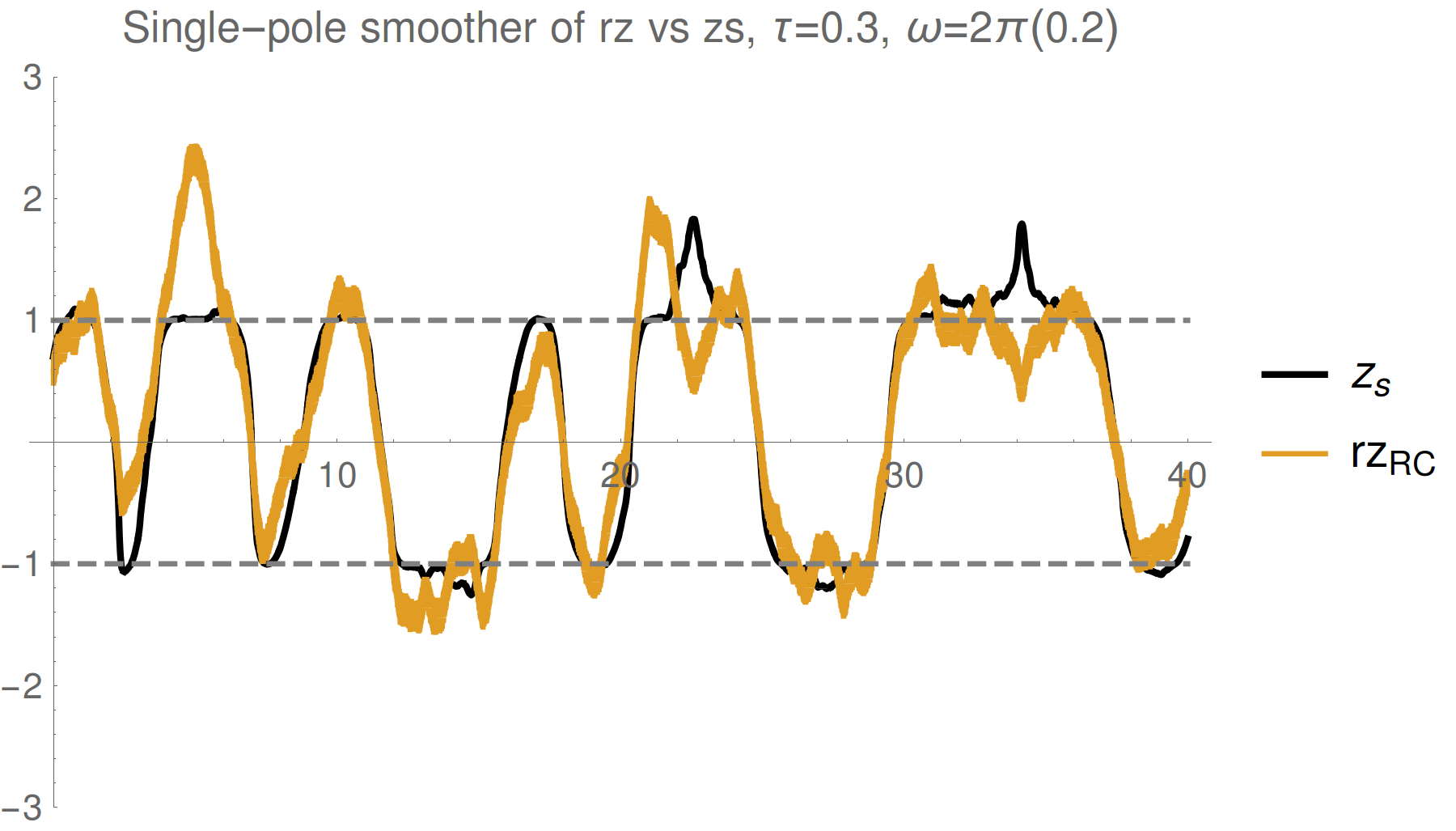
However, the collected readout follows a shifted mean value
(Consequence of the measurement backaction producing non-Markovian correlations)
The mean is the expectation value of Z only on the boundary, with unknown future record (as appropriate for simulation)
Smoothed Observable Estimate
r(t) = z_s(t) + \sqrt{\tau}\,\xi(t)
Optimally filtering/smoothing a single collected readout
will remove the Gaussian noise, and recover the
shifted observable value, not the expectation value
z_s = z_w\, \left[\frac{2}{(1+e^{-dt/2\tau}) + z_c\,(1-e^{-dt/2\tau})}\right] \approx z_w
Weak regime
Strong regime
\displaystyle z_w = \mathrm{Re}\frac{\mathrm{Tr}[E_{\vec{r}_{\mathrm{future}}}\,Z\,\rho_{\vec{r}_{\mathrm{past}}}]}{\mathrm{Tr}[E_{\vec{r}_{\mathrm{future}}}\,\rho_{\vec{r}_{\mathrm{past}}}]}
Smoothed (shifted) observable mean:
Depends on a weak value and a quadratric correction:
\displaystyle z_c = \frac{\mathrm{Tr}[E_{\vec{r}_{\mathrm{future}}}\,Z\,\rho_{\vec{r}_{\mathrm{past}}}\,Z]}{\mathrm{Tr}[E_{\vec{r}_{\mathrm{future}}}\,\rho_{\vec{r}_{\mathrm{past}}}]}
\rho_{\vec{r}_{\mathrm{past}}} = \mathcal{M}_{\vec{r}_{\mathrm{past}}}[\rho_0]
E_{\vec{r}_{\mathrm{future}}} = \mathcal{M}^*_{\vec{r}_{\mathrm{future}}}[1]
Non-Markovian dependence on both
past state and future effect matrix:
Consistent with:
Aharonov PRL 60, 1351 (1988), Wiseman PRA 65, 032111 (2002), Tsang PRL 102, 250403 (2009), Dressel PRL 104, 240401 (2010), Dressel PRA 88, 022107 (2013), Mølmer PRL 111, 160401 (2013)
( No additional ad hoc postselection)
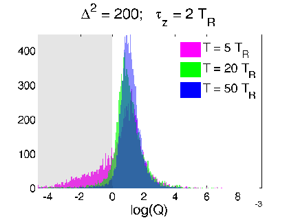
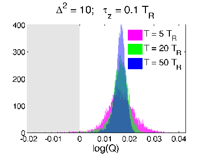
Reduced RMS Error from Readout
Is this really true? This smoothed value seems strange - can exceed eigenvalue range
Verification 1: look at relative RMS error of
both estimates compared to raw readout
Optimal filters/smoothers (Weiner, Kalman, etc.) are often defined to minimize the RMS error between a smooth dynamical estimate and the raw noisy signal
\displaystyle \log(Q) \equiv \log\frac{||z - r||}{||z_s - r||}
Discriminator:
(>0 implies smoothed value follows readout better than expectation value)
T_R : \mathrm{Rabi\, period}
\Delta^2 : \tau_z/dt
Strong regime
Weak regime
T : \mathrm{traj.\,length}
smoothed better
Yes. The smoothed value is objectively better by the same metric used for finding classical filters/smoothers.
Hypothesis Test from Readout
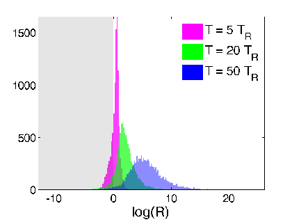
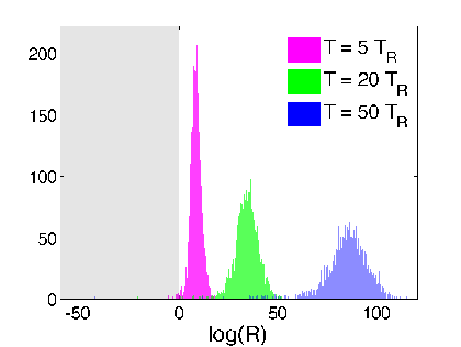
Verification 2: look at relative log-likelihood of
generating the raw readout from adding Gaussian noise to the two estimates - equivalent to a hypothesis test
\displaystyle \log(R) \equiv \log\frac{P(r|z)}{P(r|z_s)}
Discriminator:
(>0 implies smoothed value more likely than expectation value to generate readout)
T_R : \mathrm{Rabi\, period}
\Delta^2 : \tau_z/dt
Strong regime
Weak regime
T : \mathrm{traj.\,length}
smoothed better
Yes. The smoothed value is objectively more likely to generate the observed readout from additive noise
z
z_s
Corroboration by Third Party
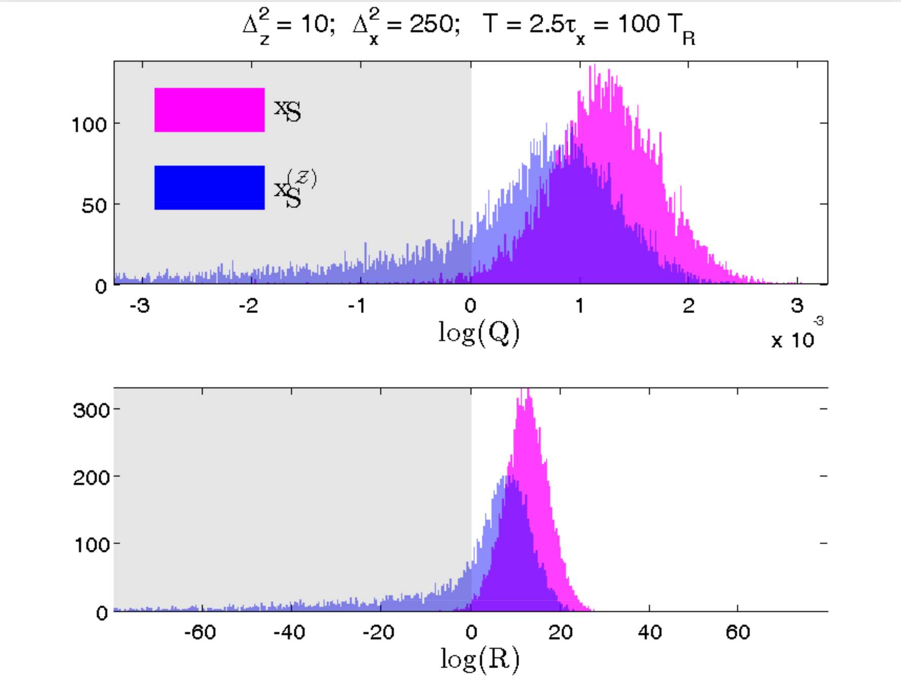
Variation: Suppose Bob is weakly monitoring a different observable (X) at the same time
If Alice is more strongly monitoring (Z) and has no access to Bob's record, does her smoothed estimate of X (not measured by her) still correspond to Bob's record?
Yes. Even without access to Bob's record, Alice can construct a smoothed estimate from her record that fits Bob's observed record better than the expectation value (computed either from Alice's subjective state or the most pure state with perfect knowledge of both records)
Test verifies that a better model of the relevant dynamics produces an objectively closer fit to the collected record
Smoothed estimate is operationally meaningful
RMS Error Test
Hypothesis Test
Blue : Alice does not know Bob's record
Pink : Alice knows both records
smoothed better
[Similar question to Guevara, Wiseman PRL 115, 180407 (2015) ]
Conclusions
z
z_s
- The mean of a single collected readout tracks a smoothed observable estimate (~ a weak value) due to backaction-correlations
- Both RMS error and hypothesis tests confirm this statement, even for a second party that is simultaneously monitoring the system
Practical Implication:
- Filtering/smoothing the readout can only approximate a usual state trajectory
- Better idea: construct smoothed observable estimate from raw record and then verify it with the filtered/smoothed record -- potential route forward for trajectory model verification without additional tomography data
Thank you!
What does a continuously monitored qubit readout really show?
By Justin Dressel
What does a continuously monitored qubit readout really show?
For continuous measurements of a quantum observable it is widely recognized that the measurement output approximates the expectation value of the observable, hidden by additive white noise. Filtering the measurement readout can thus approximately uncover the dynamics of the expectation value, during a single realization. However, using information from the entire output history yields a different, smoothed, observable estimate. We derive the form of this smoothed estimate and show that the observed readout quantitatively tracks it with higher fidelity than the expectation value during a single realization, making it an objectively meaningful quantity. In the weak measurement limit this smoothed estimate approximates a weak value, with no need for additional postselection.


