Mean-field description

of some

Deep Neural Networks

What do deep neural nets do?

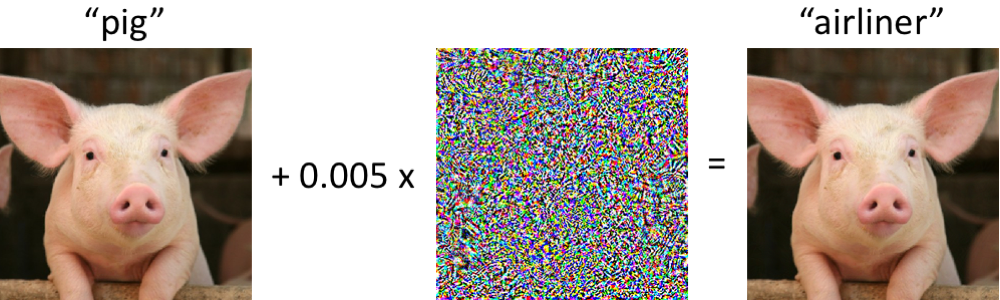
Serious mistakes when "sabotaged"

Source: http://gradientscience.org/intro_adversarial/

What you will learn today

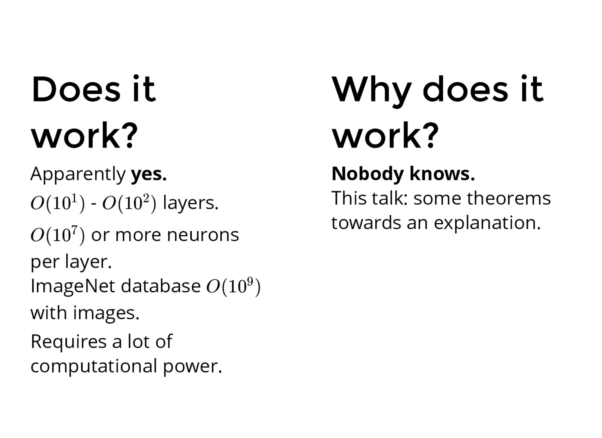
1. We do not know how/when deep nets learn.
2. At the end of the talk, we will still not know...
3. ... but we will get a glimpse of what kind of mathematical model we should use to describe the networks.

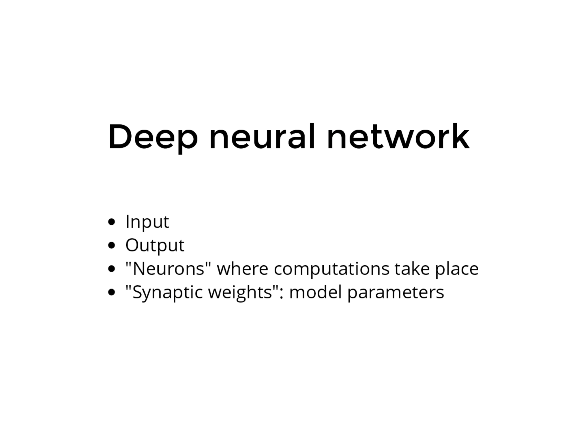
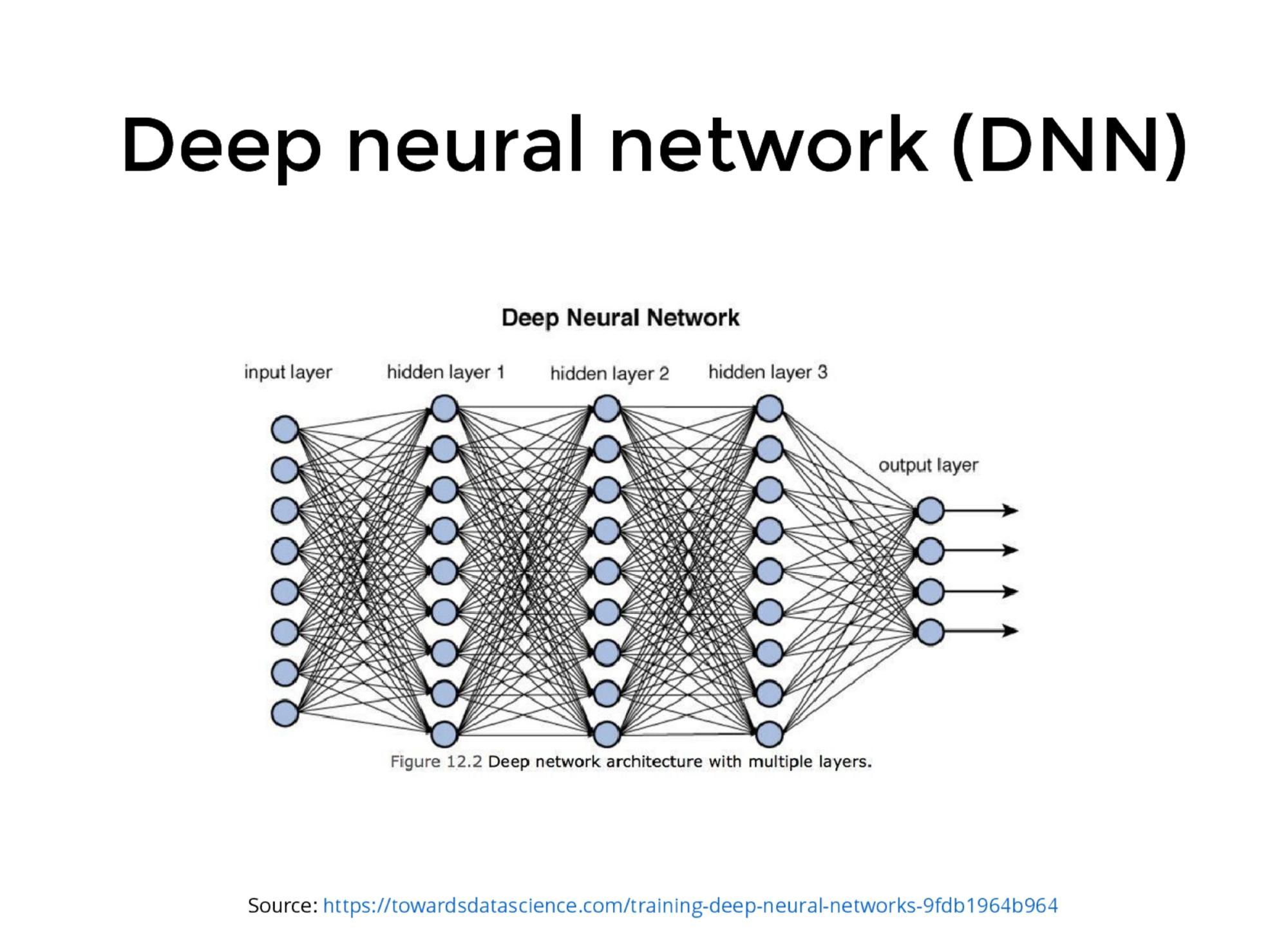
What is a deep neural network?

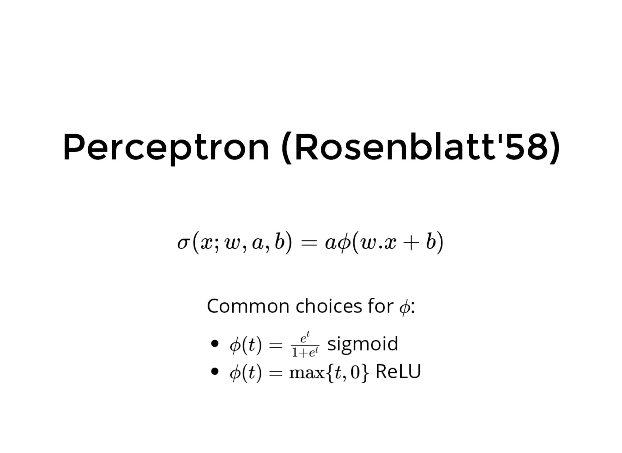
Intuition

\(x_1\)

\(x_1\)

\(x_2\)

\(x_3\)

Input

\(x_3\)

\(w_1\)

\(w_1\)

\(w_2\)

\(w_3\)

\(a,b\)

Weights

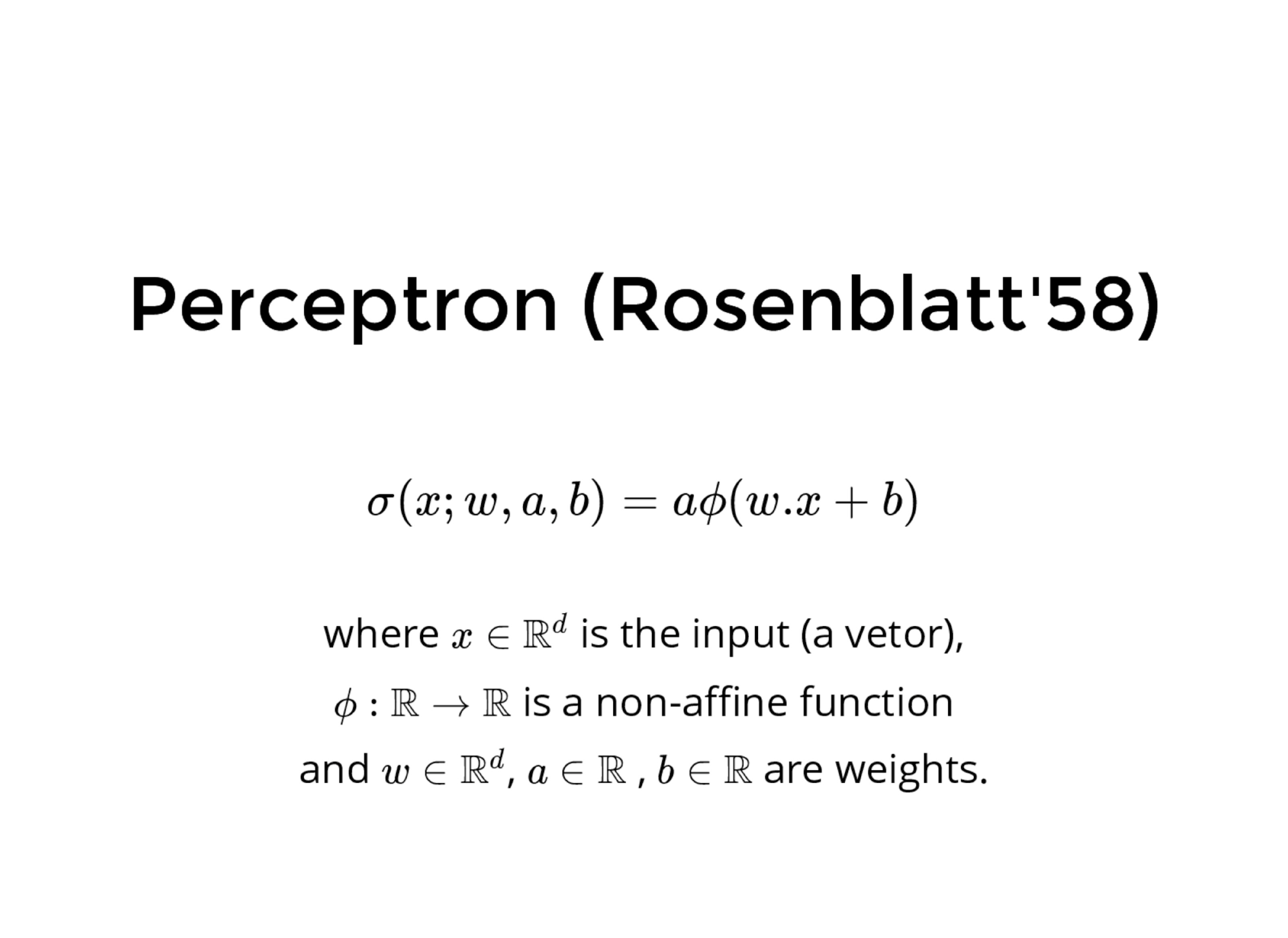
\(a\phi(x_1w_1 + x_2w_2 + x_3w_3 + b)\)

Output

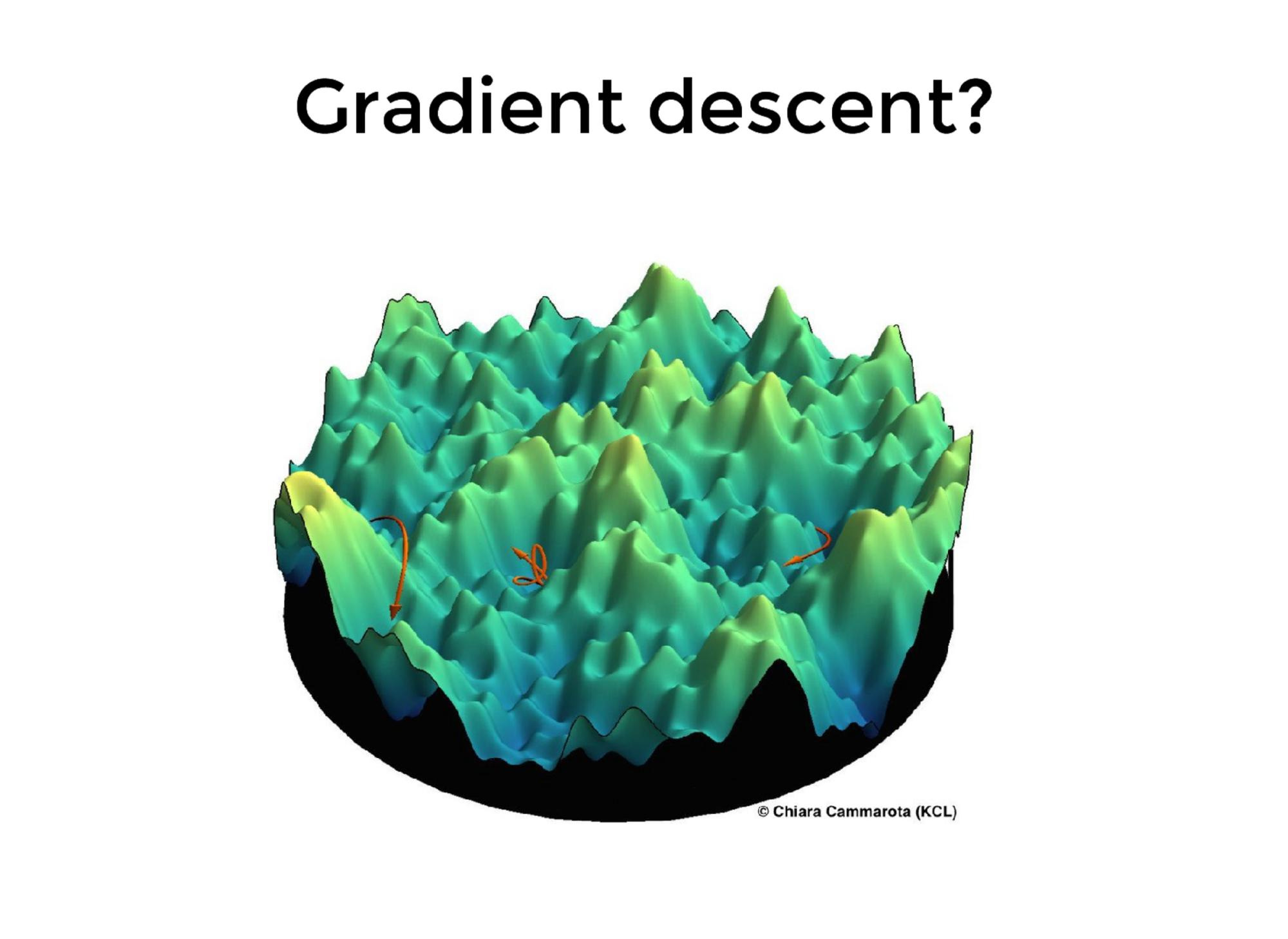
Do we really minimize error?

Tradeoff looks like this (?)

"Double descent" curve

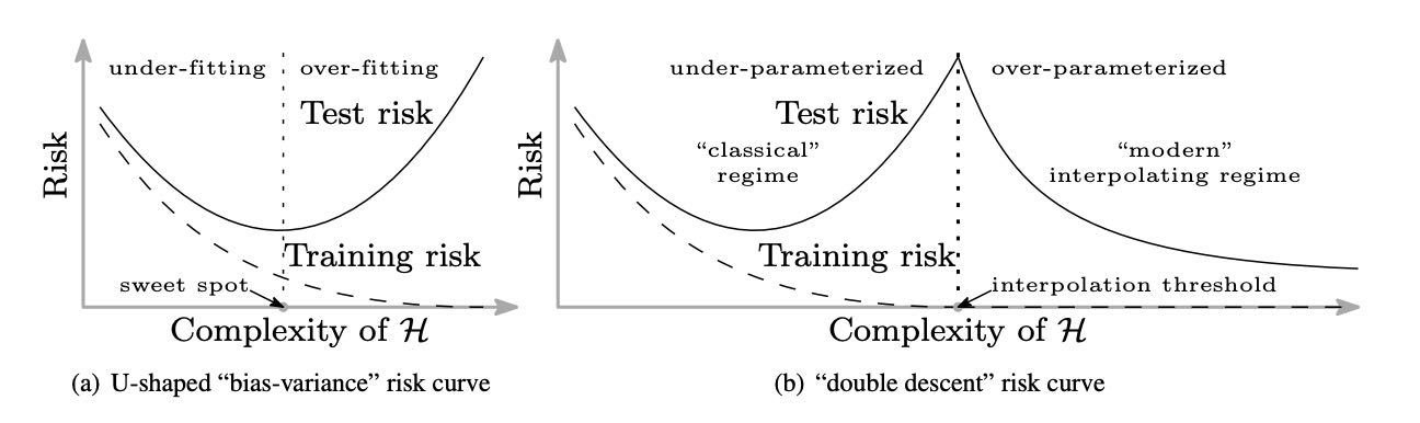
Source: https://arxiv.org/abs/1812.11118

Belkin, Hsu, Ma & Mandal (2018)

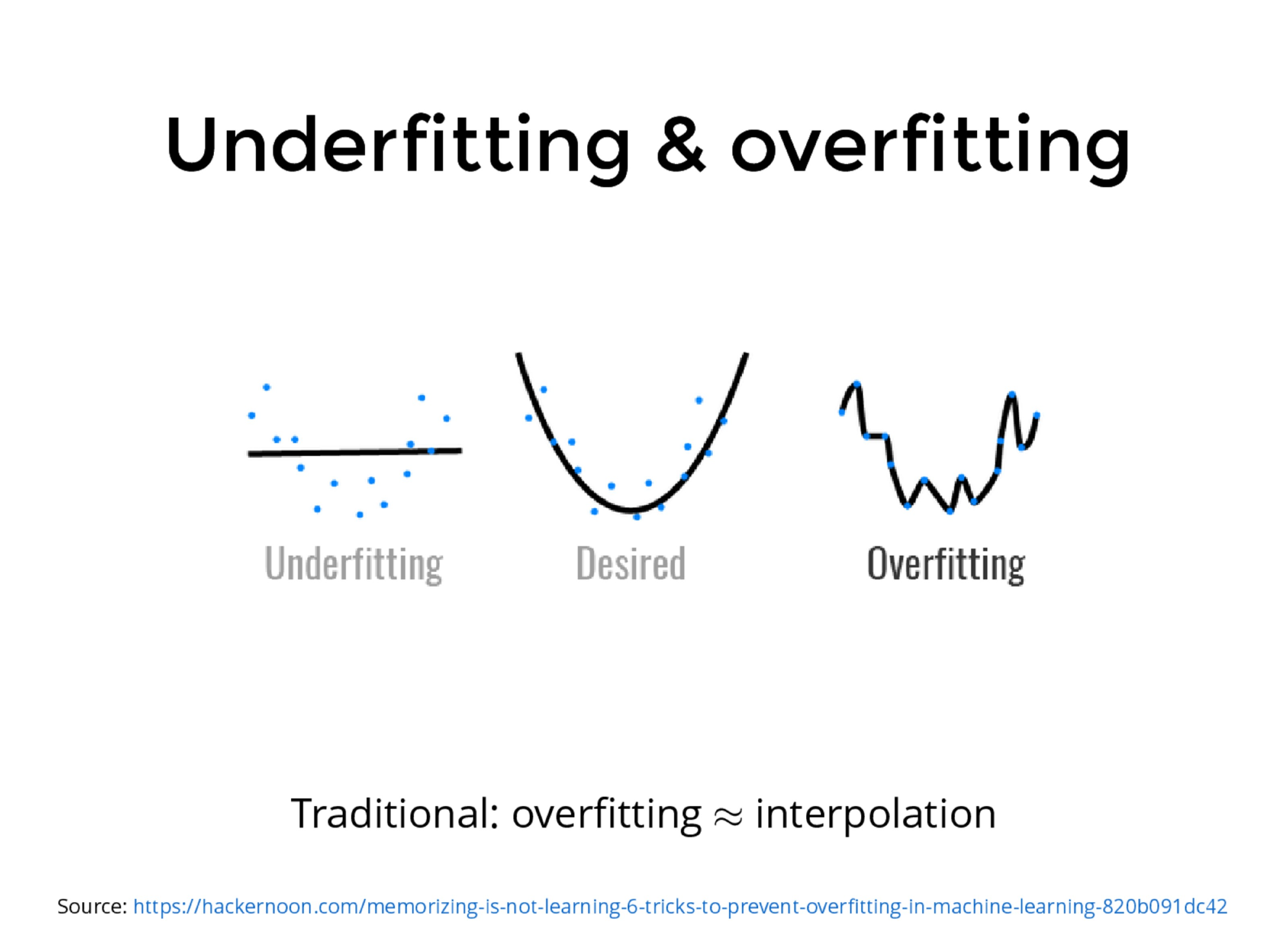
Regularized interpolation?

• Regularization = avoid or penalize complex models
• In practice, many "overparameterized" models seem to "regularize themselves" by looking for "the simplest interpolant".

(Bartlett, Belkin, Lugosi, Mei, Montanari, Rakhlin, Recht, Zhang...)

Working assumptions

• We should look for a limiting object for a network with a diverging number of parameters.
• First step: understanding what happens to the DNN when trained.

Our goal today

To understand the training of a DNN via gradient descent.

(One day: understand limit)

A first glimpse

• Consider functions that are compositions of things of the form that a DNN computes in the limit.

\(x\mapsto h_{P}(x):= \int\,h(x,\theta)\,dP(\theta)\) where \(P\in M_1(\mathbb{R}^{D})\).

• A DNN is like a composition of such functions that tries to learn "optimal parameters" \(P\). 

Our networks

Independent random initialization of weights

Our networks

Independent random initialization of weights

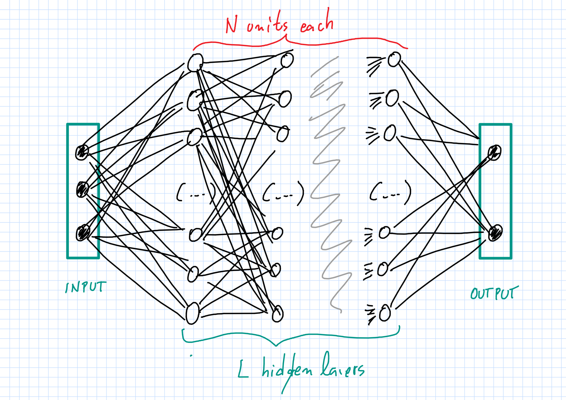
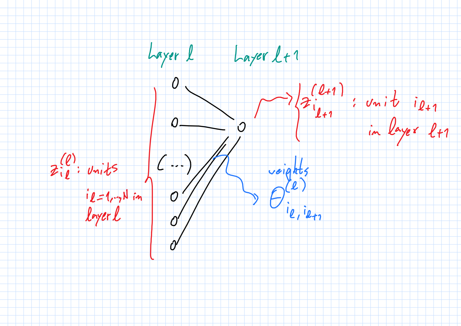
The network: layers & units

Layers \(\ell=0,1,\dots,L,L+1\):

• \(\ell=0\) input and \(\ell=L+1\) output;
• \(\ell=1,\dots,L\) hidden layers.

Each layer \(\ell\) has \(N_\ell\) units of dimension \(d_\ell\).

• \(N_0 = N_{L+1}=1\), one input \(+\) one output unit;
• \(N_\ell=N\gg 1 \) neurons in hidden layers, with \(1\leq \ell\leq L\).

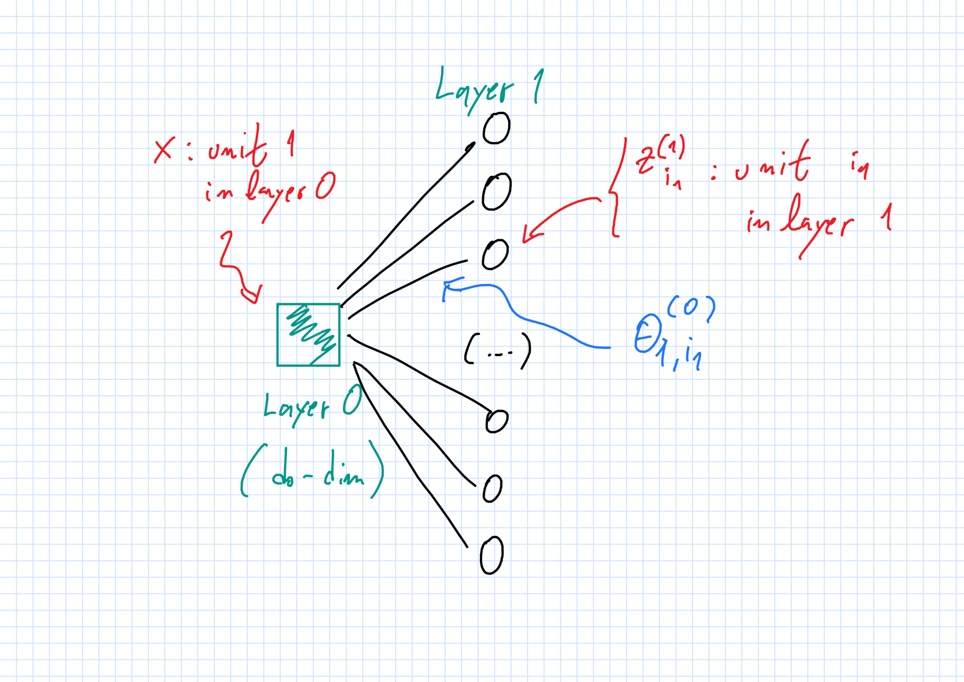
The network: weights

"Weight"  \(\theta^{(\ell)}_{i_\ell,i_{\ell+1}}\in\mathbb{R}^{D_\ell}\):

• \(i_\ell\)-th unit in layer \(\ell\) \(\to\) \(i_{\ell+1}\)-th unit in layer \(\ell+1\).

​Full vector of weights: \(\vec{\theta}_N\).

Initialization:

• all weights are independent random variables;
• weights with superscript \(\ell\) have same law \(\mu^{(\ell)}_0\).

First hidden layer

Hidden layers \(2\leq \ell\leq L\)

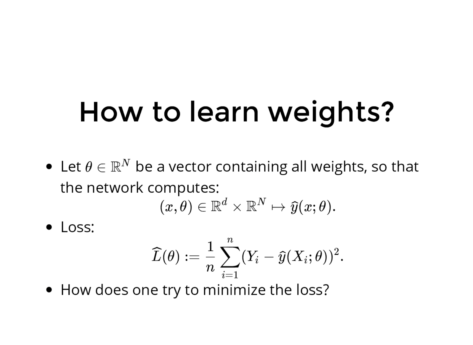
Function & loss

At output layer \(L+1\), \(N_{L+1}=1\).

Weights evolve via SGD

Weights close to input \(A_{i_1}:=\theta^{(0)}_{1,i_1}\) and output \(B_{i_L}:=\theta^{(L)}_{i_L,1}\) are not updated ("random features").

All other weights \(\theta^{(\ell)}_{i_\ell,i_{\ell+1}}\) (\(1\leq \ell\leq L-1)\): SGD with step size \(\epsilon\) and fresh samples at each iteration.

For \(\epsilon\ll 1\), \(N\gg 1\), after change in time scale, same as:

\[\frac{d}{dt}\vec{\theta}_N(t) \approx -N^2\, \nabla L_N(\vec{\theta}_N(t))\]

(\(N^2\) steps of SGD \(\sim 1\) time unit in the limit)

Limiting behavior when \(N\to+\infty, \epsilon\to 0\)

Limiting laws of the weights

Assume \(L\geq 3\) hidden layers + technicalities.

One can couple the weights \(\theta^{(\ell)}_{i_\ell,i_{\ell+1}}(t)\) to certain limiting random variables \(\overline{\theta}^{(\ell)}_{i_\ell,i_{\ell+1}}(t)\) with small error:  

Limiting random variables coincide with the weights at time 0. They also satisfy a series of properties we will describe below. 

Dependence structure

Full independence except at 1st and Lth hidden layers:

The following are all independent from one another.

1. \(\overline{\theta}_{1,i}^{(1)}(t)\equiv A_i\) (random feature weights);
2. \(\overline{\theta}_{j,1}^{(L)}(t)\equiv B_j\) (random output weights); and
3. \(\overline{\theta}^{(\ell)}_{i_\ell,i_{\ell+1}} [0,T]\) with \(2\leq \ell \leq L\) (weight trajectories).

1st and Lth hidden layers are deterministic functions:

1. \(\overline{\theta}^{(1)}_{i_1,i_2}[0,T]\) \(=\) \(F^{(1)}(A_{i_1},\theta^{(1)}_{i_1,i_2}(0))\)
2. \(\overline{\theta}^{(L)}_{i_L,i_{L+1}}[0,T]\)\(=\) \(F^{(L)}(B_{i_{L+1}},\theta^{(L)}_{i_L,i_{L+1}}(0))\)

Dependencies along a path

Distribution \(\mu_t\) of limiting weights along a path at time \(t\),

\[(A_{i_1},\overline{\theta}^{(1)}_{i_1,i_2}(t),\overline{\theta}^{(2)}_{i_2,i_3}(t),\dots,\overline{\theta}^{(L)}_{i_L,i_{L+1}}(t),B_{i_{L+1}})\sim \mu_t\]

has the following factorization into independent components:

\[\mu_t = \mu^{(0,1)}_t\otimes \mu^{(2)}_t \otimes \dots \otimes \mu_{t}^{(L-1)}\otimes \mu_t^{(L,L+1)}.\]

Contrast with time 0 (full product).

The limiting function & loss

At any time \(t\), the loss of function \(\widehat{y}(x,\vec{\theta}_N(t))\) is approximately the loss composition of functions of the generic form \(\int\,h(x,\theta)\,dP(\theta)\). Specifically,

\[L_N(\vec{\theta}_N)\approx \frac{1}{2}\mathbb{E}_{(X,Y)\sim P }\,\|Y - \overline{y}(X,\mu_t)\|^2\] where

Where is this coming from?

Limit evolution of weights

1. Form of drift depends only on layer of the weight.
2. Involves the weight itself, the densities of weights in other layers and (for \(\ell=1,L\)) nearby weights.

Laws of large numbers

McKean-Vlasov structure

Ansatz:

1. Terms involving a large number of random weights can be replaced by interactions with their density.
2. The densities only depend on the layer of the weight.

\(\Rightarrow\) McKean-Vlasov type of behavior.

McKean Vlasov

processes?

Abstract McKean-Vlasov

Consider:

1. \(M_1(\mathbb{R}^D)\) = all prob. distributions over \(R^D\),
2. measures \(\mu_t\in M_1(\mathbb{R}^D)\) for \(t\geq 0\);
3. noise level \(\sigma\geq 0\);
4. drift function \(\psi:\mathbb{R}\times \mathbb{R}^D\times M_1(\mathbb{R}^D)\to \mathbb{R}^D\);
5. A random trajectory:

Self-consistency: \(Z(t)\sim \mu_t\) for all times \(t\geq 0\)

Existence and uniqueness

Under reasonable conditions, for any initial measure \(\mu_0\) there exists a unique trajectory

\[t\geq 0\mapsto \mu_t\in M_1(\mathbb{R}^D)\]

such that any random process \(Z\) satisfying

satisfies the McKean-Vlasov consistency property:

\[Z(t)\sim \mu_t, t\geq 0.\]

[McKean'1966, Gärtner'1988, Sznitman'1991, Rachev-Ruschendorf'1998,...]

PDE descripition

Density \(p(t,x)\) of \(\mu_t\) evolves according to a (possibly) nonlinear PDE.

nonlinearity comes from \(\mu_t\sim p(t,x)\)

Mei - Montanari - Nguyen

Function computed by network:

\[\widehat{y}(x,\vec{\theta}_N) = \frac{1}{N}\sum_{i=1}^N\sigma_*(x,\theta_i).\]

Loss:

\[L_N(\vec{\theta}_N):=\frac{1}{2}\mathbb{E}_{(X,Y)\sim P}(Y-\widehat{y}(X,\vec{\theta}_N))^2\]

Mei - Montanari - Nguyen 

Evolution of particle \(i\) in the right time scale:

where

\[\widehat{\mu}_{N,t}:= \frac{1}{N}\sum_{i=1}^N \delta_{\theta_i(t)}.\]

Informal derivation

Assume a LLN holds and a deterministic limiting density \[\widehat{\mu}_{N,t}\to \mu_t\] emerges for large \(N\). Then particles should follow:

In particular, independence at time 0 is preserved at all times. Also limiting self consistency:

Typical \(\theta_i(t)\sim \widehat{\mu}_{N,t}\approx \mu_t\).

Mean-field particle systems

Meta-theorem:

Consider a system of \(N\gg 1\) evolving particles with mean field interactions.

If no single particle "prevails", then the thermodynamic limit is a McKean-Vlasov process.

Important example: 

Mei-Montanari-Nguyen for networks with \(L=1\).

A "coupling" construction

Let \(\mu_t,t\geq 0\) be the McK-V solution to

\[Z(0)\sim \mu_0, \frac{d}{dt}Z(t) = \psi(Z(t),\mu_t),Z(t)\sim \mu_t.\]

Now consider trajectories \(\overline{\theta}_i[0,T]\) of the form:

\[\overline{\theta}_i(0):=\theta_i(0),\; \frac{d}{dt}\overline{\theta}_i(t) = \psi(\overline{\theta}_i(t),\mu_t).\]

Then:

\[\mathbb{E}|\theta_i(t) - \overline{\theta}_i(t)|\leq Ce^{CT}\,(\epsilon + (D/N)^{1/2}).\]

Main consequence

At any time \(t\geq 0\),

\[|L_N(\vec{\theta}_N(t)) - L(\mu_t)| \leq C_t\,(\epsilon + N^{-1/2}),\]

where, for \(\mu\in M_1(\mathbb{R}^d)\),

\[L(\mu) = \frac{1}{2}\mathbb{E}_{(X,Y)\sim P}\left(Y - \int_{\R^d}\,\sigma_*(X,\theta)\,d\mu(\theta)\right)^2.\]

Structure of PDE

Density \(p(t,x)\) of \(\mu_t\) evolves according to a (possibly) nonlinear PDE.

In their case, this corresponds to a 

gradient flow with convex potential in the space of probability measures over \(\R^D\).

Ambriosio, Gigli, Savaré, Figalli, Otto, Villani...

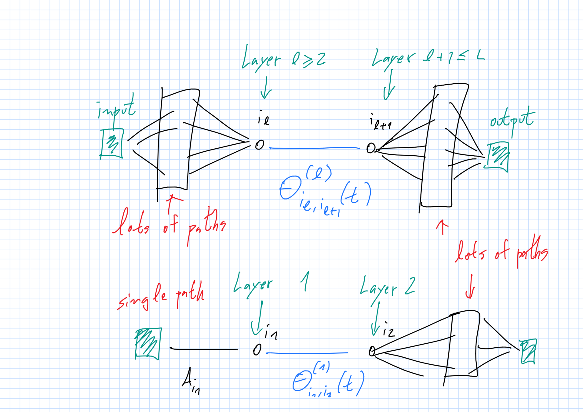
What about our setting?

Dependencies in our system are trickier.

• Before: basic units = individual weights.

Remain i.i.d. at all times when \(N\gg 1\). Direct connection between system and i.i.d. McK-V trajectories.

• Now: basic units are paths.

Will not have i.i.d. trajectories even in the limit because the paths intersect. Also, McK-V is discontinuous due to conditioning appearing in the drifts. 

What saves the day:

dependencies we expect from the limit are manageable.

Many paths \(\Rightarrow\) LLN

Finding the right McKean-Vlasov equation

Deep McK-V: activations

Recursion at time t:

Deep McK-V: activations

Recursion at time t for \(\ell=2,3,\dots,L+1\):

Deep McK-V: backprop

Backwards recursion:

Recall \(\widehat{y}(x,\vec{\theta}_N)=\sigma^{(L+1)}(z^{(L)}_1(x,\vec{\theta}_N))\). Define:

Deep McK-V: backprop

Limiting version:

For \(\ell\leq L-2\), define:

Deep McK-V: backprop

For \(2\leq \ell\leq L-2\), backprop formula:

is replaced in the evolution of \(\overline{\theta}^{(\ell)}_{i_\ell,i_{\ell+1}}\) by:

\[\overline{M}^{(\ell+1)}(x,t)\,D_\theta\sigma^{(\ell)}_*(\overline{z}^{(\ell)}(x,t),\overline{\theta}^{(\ell)}_{i_\ell,i_{\ell+1}}(t))\]

Deep McK-V: the upshot

For \(2\leq \ell\leq L-2\), the time derivative of \(\overline{\theta}^{(L)}(t)\) should take the form

where the \(\overline{z}\) are determined by the marginals:

Deep McK-V: proof (I)

Find unique McK-V process \((\mu_t)_{t\geq 0}\) that should correspond to weights on a path from input to output:

\[(A_{i_1},\theta^{(1)}_{i_1,i_2}(t),\dots,\theta^{(L-1)}_{i_{L-1},i_{L}}(t),B_{i_{L}})\approx \mu_t.\]

Prove that trajectories have the right dependency structure.

\[\mu_{[0,T]} = \mu^{(0,1)}_{[0,T]}\otimes \mu^{(2)}_{[0,T]} \otimes \mu_{[0,T]}^{(L-1)}\otimes \mu_{[0,T]}^{(L,L+1)}.\]

Deep McK-V: proof (II)

Populate the network with limiting weight trajectories:

1. I.i.d. part:

Generate i.i.d. random variables: \[A_{i_1}\sim \mu_0^{(0)},B_{i_L}\sim \mu^{(L+1)}_0, \overline{\theta}_{i_\ell,i_{\ell+1}^{(\ell)}([0,T])}\sim \mu^{(\ell)}_{[0,T]}\,(2\leq \ell\leq L-2)\]

2. Conditionally independent part:

For each pair \(i_1,i_2\), generate \(\theta^{(1)}_{i_1,i_2}([0,T])\) from the conditional measure \(\mu^{(0,1)}_{[0,T]}\) given the weight \(A_{i_1}\). Similarly for weights \(\theta^{(L-1)}_{i_{L-1},i_L}\).

Deep McK-V: proof (III)

The limiting weights we generated coincide with true weights at time 0. From McK-V drift conditions, can check via Gronwall's inequality that limiting and true weights are close.

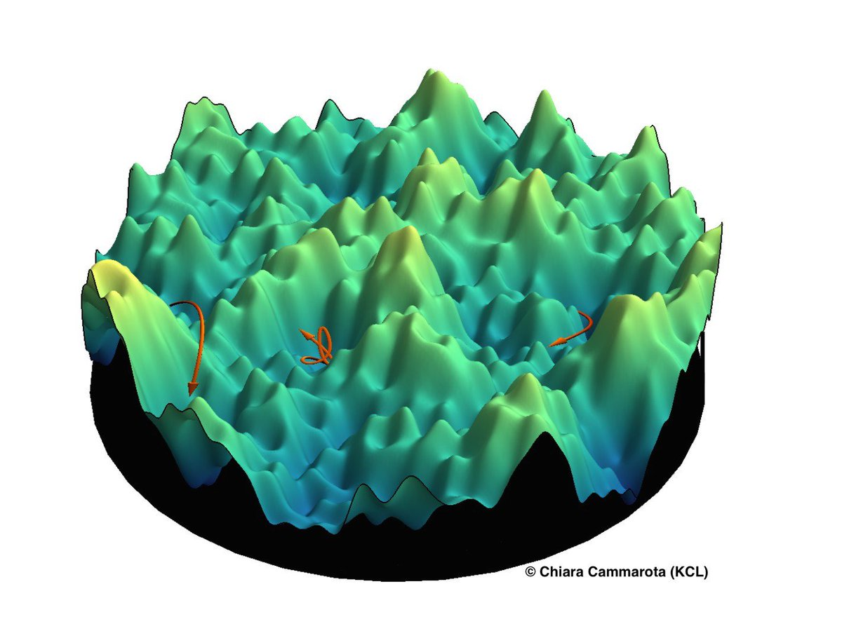
Limiting system of McKean-Vlasov PDEs

It looks like this.

[Public domain/Wikipedia]

Problems & extensions

What goes wrong if weights close to input and output are allowed to change over time?

Not much.

A "blank slate"

• Consider functions that are compositions of things of the form that a DNN computes in the limit.

\(x\mapsto h_{P}(x):= \int\,h(x,\theta)\,dP(\theta)\) where \(P\in M_1(\mathbb{R}^{D})\).

• What other methods can be used to optimize the choices of the distributions \(P\)?

Thank you!