Mean-field description

of some

Deep Neural Networks

Current uses of DNNs

• Image recognition and classification
• Machine translation
• Game playing (...)

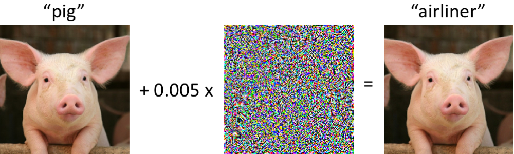
Huge improvements & lots of vulnerabilities!

Current questions 

• How does learning take place?
• What kind of regression method are they?
• So many parameters, why doesn't variance blow up?
• How do we avoid vulnerabilities?

Today

At the end of the talk, we will still not know the answers ...

... but we will get a glimpse of mathematical methods we should use to describe the networks.

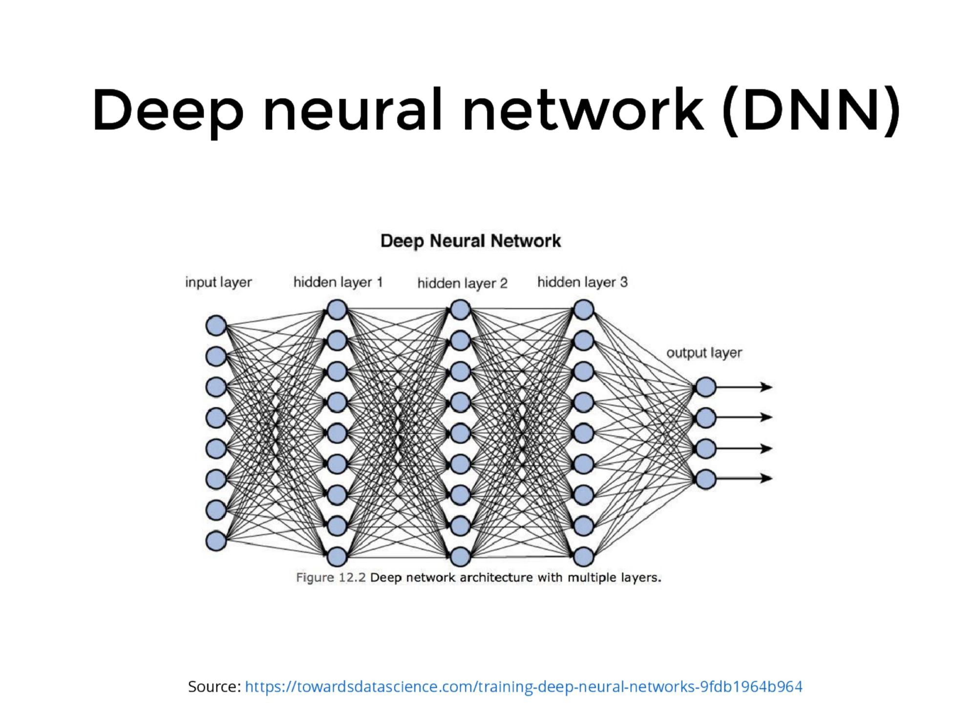
What is a deep neural network?

Perceptron = single neuron

\(x_1\)

\(x_1\)

\(x_2\)

\(x_3\)

Input

\(x_3\)

\(\theta_1\)

\(\theta_2\)

\(\theta_3\)

\(a,b\)

Weights

\(a\phi(\sum_ix_i\theta_i + b)\)

Output

(Rosenblatt'59)

Total # of parameters \(10^7\) to \(10^9 \).

Learning

Data: points \((X_i,Y_i)\stackrel{\rm i.i.d.}{\sim}\,P\)  \(\R^{d_X}\times \R^{d_Y}\).

Network: parameterized function \(\widehat{y}:\R^{d_X}\times \R^{D_N}\to \R^{d_Y}\).

Train: (stochastic online) gradient descent

\[\theta^{(k+1)} = \theta^{(k)} - \epsilon \alpha^{(k)}\,(Y_{k+1}-\widehat{y}(X_{k+1},\theta^{(k)}))^T \nabla_\theta \widehat{y}(X_{k+1},\theta^{(k)}).\]

In expectation, this follows the gradient of loss:

\[L(\theta):=\frac{1}{2}\mathbb{E}_{(X,Y)\sim P}\|Y - \widehat{y}(X,\theta)\|^2 .\]

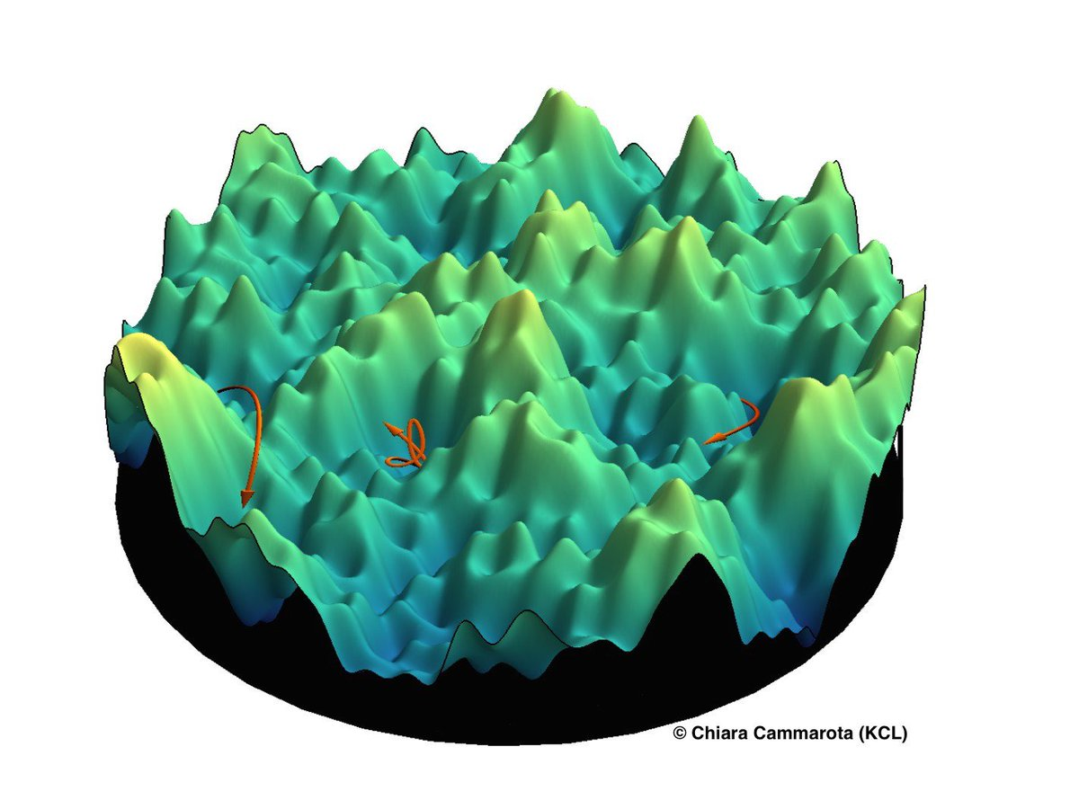
Does it converge to a min?

"Double descent" for

bias-variance tradeoff

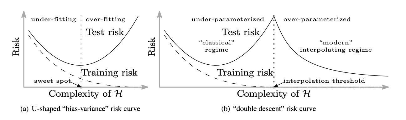
Source: https://arxiv.org/abs/1812.11118

Belkin, Hsu, Ma & Mandal (2018)

Working assumptions

• We should look for a limiting object for a network with a diverging number of parameters (*)
• First step: understanding what happens to the DNN when trained.

(*) See Ongie, Willett, Soudry & Srebo https://arxiv.org/abs/1910.01635

A first glimpse

• Consider functions that are compositions of things of the form that a DNN computes in the limit.

\(x\mapsto h_{\mu}(x):= \int\,h(x,\theta)\,d\mu(\theta)\) where \(\mu\in M_1(\mathbb{R}^{D})\).

• A DNN is like a composition of such functions that tries to learn "optimal parameters" \(\mu\) for each layer via gradient descent. 

Our networks

Independent random initialization of weights

Our networks

Independent random initialization of weights

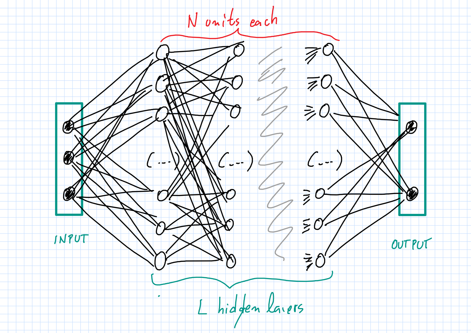
The network: layers & units

Layers \(\ell=0,1,\dots,L,L+1\):

• \(\ell=0\) input and \(\ell=L+1\) output;
• \(\ell=1,\dots,L\) hidden layers.

Each layer \(\ell\) has \(N_\ell\) units of dimension \(d_\ell\).

• \(N_0 = N_{L+1}=1\), one input \(+\) one output unit;
• \(N_\ell=N\gg 1 \) neurons in hidden layers, with \(1\leq \ell\leq L\).

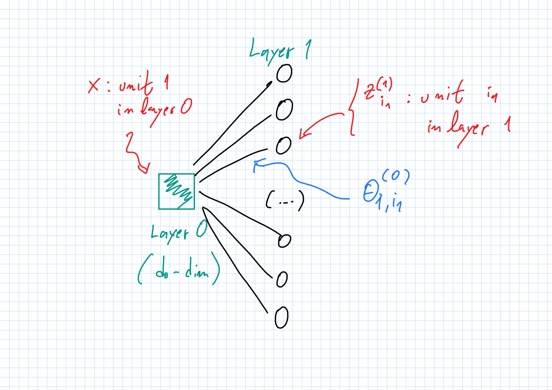
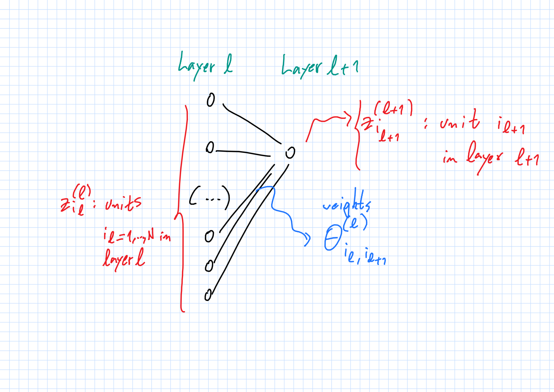
The network: weights

"Weight"  \(\theta^{(\ell)}_{i_\ell,i_{\ell+1}}\in\mathbb{R}^{D_\ell}\):

• \(i_\ell\)-th unit in layer \(\ell\) \(\to\) \(i_{\ell+1}\)-th unit in layer \(\ell+1\).

​Full vector of weights: \(\vec{\theta}_N\).

Initialization:

• all weights are independent random variables;
• weights with superscript \(\ell\) have same law \(\mu^{(\ell)}_0\).

First hidden layer

Hidden layers \(2\leq \ell\leq L\)

Function & loss

At output layer \(L+1\), \(N_{L+1}=1\).

Limiting behavior when \(N\to+\infty, \epsilon\to 0\)

Limiting laws of the weights

Assume \(L\geq 3\) hidden layers + technicalities on \(\sigma\).

One can couple the weights \(\theta^{(\ell)}_{i_\ell,i_{\ell+1}}(t)\) to certain limiting random variables \(\overline{\theta}^{(\ell)}_{i_\ell,i_{\ell+1}}(t)\) with small error:  

Limiting random variables coincide with the weights at time 0 & satisfy a series of properties we will now describe. 

Dependence structure

Full independence except at 1st and Lth hidden layers:

The following are all independent from one another.

1. \(\overline{\theta}_{1,i}^{(1)}(t)\equiv A_i\) (random feature weights);
2. \(\overline{\theta}_{j,1}^{(L)}(t)\equiv B_j\) (random output weights); and
3. \(\overline{\theta}^{(\ell)}_{i_\ell,i_{\ell+1}} [0,T]\) with \(2\leq \ell \leq L\) (weight trajectories).

1st and Lth hidden layers are deterministic functions:

1. \(\overline{\theta}^{(1)}_{i_1,i_2}[0,T]\) \(=\) \(F^{(1)}(A_{i_1},\theta^{(1)}_{i_1,i_2}(0))\)
2. \(\overline{\theta}^{(L)}_{i_L,i_{L+1}}[0,T]\)\(=\) \(F^{(L)}(B_{i_{L+1}},\theta^{(L)}_{i_L,i_{L+1}}(0))\)

Dependencies along a path

Distribution \(\mu_t\) of limiting weights along a path at time \(t\),

\[(A_{i_1},\overline{\theta}^{(1)}_{i_1,i_2}(t),\overline{\theta}^{(2)}_{i_2,i_3}(t),\dots,\overline{\theta}^{(L)}_{i_L,i_{L+1}}(t),B_{i_{L+1}})\sim \mu_t\]

has the following factorization into independent components:

\[\mu_t = \mu^{(0,1)}_t\otimes \mu^{(2)}_t \otimes \dots \otimes \mu_{t}^{(L-1)}\otimes \mu_t^{(L,L+1)}.\]

Contrast with time 0 (full product).

The limiting function & loss

At any time \(t\), the loss of function \(\widehat{y}(x,\vec{\theta}_N(t))\) is approximately the loss composition of functions of the generic form \(\int\,h(x,\theta)\,dP(\theta)\). Specifically,

\[L_N(\vec{\theta}_N)\approx \frac{1}{2}\mathbb{E}_{(X,Y)\sim P }\,\|Y - \overline{y}(X,\mu_t)\|^2\] where

Where is this coming from?

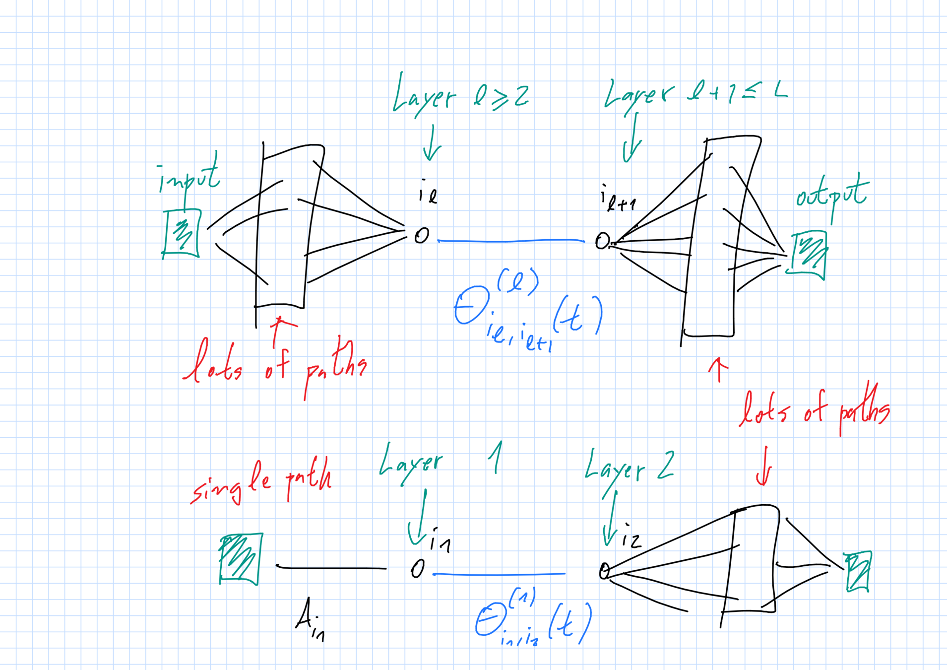
Backprop & McKean-Vlasov

Backpropagation (Hinton?): chain rule describes partial derivatives as sums of paths going back and forward in the network

Ansatz: Terms involving a large number of random weights can be replaced by interactions with their density (a law of large numbers).

\(\Rightarrow\) McKean-Vlasov type of behavior.

Abstract McKean-Vlasov

Consider:

1. \(M_1(\mathbb{R}^D)\) = all prob. distributions over \(R^D\),
2. measures \(\mu_t\in M_1(\mathbb{R}^D)\) for \(t\geq 0\);
3. noise level \(\sigma\geq 0\);
4. drift function \(\psi:\mathbb{R}\times \mathbb{R}^D\times M_1(\mathbb{R}^D)\to \mathbb{R}^D\);
5. A random trajectory:

Self-consistency: \(Z(t)\sim \mu_t\) for all times \(t\geq 0\)

Structure of PDE

Density \(p(t,x)\) of \(\mu_t\) evolves according to a (possibly) nonlinear PDE.

In the case of shallow (\(L=1\)) nets, this corresponds to a 

gradient flow with convex potential in the space of probability measures over \(\R^D\).

Ambriosio, Gigli, Savaré, Figalli, Otto, Villani...

Shallow vs deep nets

Shallow:

Mei, Montanari & Nguyen (2018); Sirignano & Spiliopoulos (2018); Rotskoff & Vanden Einjden (2018).

"Easy case".

Deep (before us):

Modified limit by S&S (2019).

Heuristic by Nguyen (2019).

Hard case: discontinuous drift in McKean-Vlasov

New issues

Dependencies in our system are trickier.

• Before: basic units = individual weights.

Remain i.i.d. at all times when \(N\gg 1\). Direct connection between system and i.i.d. McK-V trajectories.

• Now: basic units are paths.

Will not have i.i.d. trajectories even in the limit because the paths intersect. Also, McK-V is discontinuous due to conditioning appearing in the drifts. 

Many paths \(\Rightarrow\) LLN

Limiting system of McKean-Vlasov PDEs

It looks like this.

[Public domain/Wikipedia]

A "blank slate"

• Consider functions that are compositions of things of the form that a DNN computes in the limit.

\(x\mapsto h_{\mu}(x):= \int\,h(x,\theta)\,d\mu(\theta)\) where \(\mu\in M_1(\mathbb{R}^{D})\).

• What other methods can be used to optimize the choices of the distributions \(\mu\)?

Thank you!