


Sarah Dean PRO
asst prof in CS at Cornell
Sarah Dean¹ Horia Mania¹ Nikolai Matni² Ben Recht¹ Stephen Tu³
¹University of California, Berkeley ²University of Pennsylvania ³Google Brain
Classic RL setting: discrete problems and inspired by games
RL techniques applied to continuous systems interacting with the physical world
Control theory:
Optimal Control Problem:
minimize \(\mathbb{E}[\sum_{t=0}^T\)cost\((x_t, u_t)]\)
s.t. \(x_{t+1} = f_t(x_t, u_t, w_t)\)
plant
controller
state \(x\),
cost
input \(u\)
Simplest OCP: linear dynamics, quadratic cost, Gaussian process noise
minimize \(\mathbb{E}\left[ \displaystyle\lim_{T\to\infty}\frac{1}{T}\sum_{t=0}^T x_t^\top Q x_t + u_t^\top R u_t\right]\)
s.t. \(x_{t+1} = Ax_t+Bu_t+w_t\)
\(u_t = \underbrace{-(R+B^\top P B)^{-1} B^\top P A}_{K_\star}x_t\)
where \(P=\text{DARE}(A,B,Q,R)\) also defines the value function \(V(x) = x^\top P x\)
Static feedback controller is optimal and can be computed in closed-form:
How many observations are necessary to control unknown system?
As long as \(N\) is large enough, then with probability at least \(1-\delta\),
\(\mathrm{rel.~error~of}~\widehat{\mathbf K}\lesssim \frac{\mathrm{size~of~noise}}{\mathrm{size~of~excitation}} \sqrt{\frac{\mathrm{dimension}}{N} \log(1/\delta)} \cdot\mathrm{robustness~of~}K_\star\)
excitation
\((A_\star, B_\star)\)
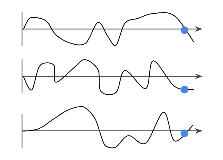
\(N\) observations
1. Collect \(N\) observations and estimate \(\widehat A,\widehat B\) and confidence intervals
2. Use estimates to synthesize robust controller \(\widehat{\mathbf{K}}\)
\((A_\star, B_\star)\)
\(\widehat{\mathbf{K}}\)
\((A_\star, B_\star)\)
Least squares estimate: \((\widehat A, \widehat B) \in \arg\min \sum_{\ell=1}^N \|Ax_{T}^{(\ell)} +B u_{T}^{(\ell)} - x_{T+1}^{(\ell)}\|^2 \)
As long as \(N\gtrsim n+p+\log(1/\delta)\), then with probability at least \(1-\delta\),
\(\|\widehat A - A_\star\| \lesssim \frac{\sigma_w}{\sqrt{\lambda_{\min}(\sigma_u^2 G_T G_T^\top + \sigma_w^2 F_T F_T^\top )}} \sqrt{\frac{n+p }{N} \log(1/\delta)} \), \(\|\widehat B - B_\star\| \lesssim \frac{\sigma_w}{\sigma_u} \sqrt{\frac{n+p }{N} \log(1/\delta)} \)
with controllability Grammians defined as
\(G_T = \begin{bmatrix}A_\star^{T-1}B_\star&A_\star^{T-2}B_\star&\dots&B_\star\end{bmatrix} \qquad F_T = \begin{bmatrix}A_\star^{T-1}&A_\star^{T-2}&\dots&I\end{bmatrix}\)
\((A_\star, B_\star)\)
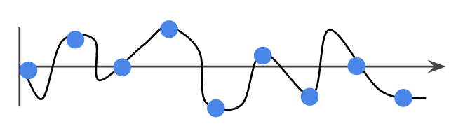
Excitation
\(u_t^{(\ell)} \sim \mathcal{N}(0, \sigma_u^2)\)
Observe states \(\{x_t^{(\ell)}\}\)
have independent Gaussian entries
\(\begin{bmatrix} x_{T}^{(\ell)} \\u_{T}^{(\ell)} \end{bmatrix} \sim \mathcal{N}\left(0, \begin{bmatrix}\sigma_u^2 G_TG_T^\top + \sigma_w^2 F_TF_T^\top &\\ & \sigma_u^2 I\end{bmatrix}\right)\)
\(w_t^{(\ell)} \sim \mathcal{N}\left(0, \sigma_w^2\right)\)
The least-squares estimate is
\(\arg \min \|Z_N \begin{bmatrix} A & B\end{bmatrix} ^\top - X_N\|^2_F = (Z_N^\top Z_N)^\dagger Z_N^\top X_N\)
\(= \begin{bmatrix} A_\star & B_\star \end{bmatrix} ^\top + (Z_N^\top Z_N)^\dagger Z_N^\top W_N\)
Data and noise matrices
\(X_N = \begin{bmatrix} x_{T+1}^{(1)} & \dots & x_{T+1}^{(N)} \end{bmatrix}^\top\)
\(Z_N = \begin{bmatrix} x_{T}^{(1)} & \dots & x_{T}^{(N)} \\u_{T}^{(1)} & \dots & u_{T}^{(N)} \end{bmatrix}^\top\)
\(W_N = \begin{bmatrix} w_{T}^{(1)} & \dots & w_{T}^{(N)} \end{bmatrix}^\top \)
lower bound minimum singular value,
or compute data-dependent bound
upper bound inner products
\(\Big\|\begin{bmatrix} \widehat A - A_\star \\ \widehat B - B_\star\end{bmatrix}\Big\| \lesssim \frac{\sigma_w}{C_u \sigma_u}\sqrt{\frac{n+p }{T} \log(d/\delta)} \)
To guarantee worst-case performance, use estimates \(\widehat A,\widehat B\) and confidence intervals for robust synthesis:
\( \underset{\mathbf u=\mathbf{Kx}}{\min}\) \(\underset{\|A-\widehat A\|\leq \varepsilon_A \atop \|B-\widehat B\|\leq \varepsilon_B}{\max}\) \(\mathbb{E}\left[\lim_{T\to\infty} \frac{1}{T}\sum_{t=0}^T x_t^\top Q x_t + u_t^\top R u_t\right]\)
s.t. \(x_{t+1} = Ax_t + Bu_t + w_t\)
To tackle this nonconvex problem, we use an alternate parametrization.
\((A,B)\)
controller \(\mathbf{K}\)
\(\bf x\)
\(\bf u\)
\(\bf w\)
\(\bf x\)
\(\bf u\)
\(\bf w\)
In closed loop, state and input are linear functions of disturbance
\(x_t = \sum_{k=0}^t A^{k}(Bu_{t-k} + w_{t-k})\)
\(u_t = \sum_{k=0}^t K_kx_{t-k}\)
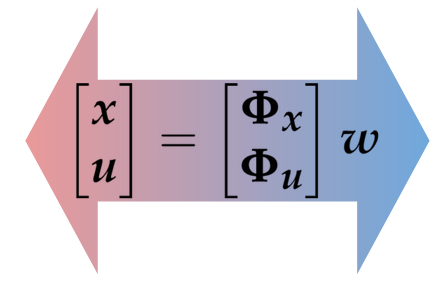
\(\begin{bmatrix} x_t\\u_t \end{bmatrix} = \sum_{k=0}^t \begin{bmatrix} \Phi_x(t)\\ \Phi_u(t) \end{bmatrix} w_{t-k}\)
Instead of reasoning about a controller \(\mathbf{K}\), we reason about the interconnection \(\mathbf\Phi\) directly.
\( \underset{\color{red}\mathbf{K}}{\min}\) \(\mathbb{E}\left[\lim_{T\to\infty} \frac{1}{T}\sum_{t=0}^T x_t^\top Q x_t + u_t^\top R u_t\right]\)
s.t. \(x_{t+1} = Ax_t + Bu_t + w_t\)
\(u_{t} = {\color{red}\mathbf{K}}(x_t)\)
\( \underset{\color{blue}\mathbf{\Phi}}{\min}\)\(\left\| \begin{bmatrix} Q^{1/2} &\\& R^{1/2}\end{bmatrix}{\color{blue} \mathbf{\Phi}} \right\|_{\mathcal{H}_2}^2\)
s.t. \( {\color{blue}\mathbf\Phi }\in\mathrm{Affine}(A, B)\)
Instead of reasoning about \(\mathbf{K}\), reason about the interconnection \(\mathbf\Phi\) directly.
\( \underset{\color{red}\mathbf{K}}{\min}\) \(\mathbb{E}\left\|\begin{bmatrix} Q^{1/2} \mathbf x\\ R^{1/2} \mathbf u\end{bmatrix}\right\|_{2}^2\)
s.t. \( z\mathbf x = A\mathbf x + B\mathbf u + \mathbf w\)
\(\mathbf u = {\color{red}\mathbf{K}}\mathbf x\)
Theorem [Anderson et al., 2019]: Correspondence between feedback controller and system response,
\({\mathbf\Phi }\in\mathrm{Affine}(A, B)\) \(\iff\) \(\mathbf K = \mathbf{\Phi_u\Phi_x}^{-1}\) achieves response \(\mathbf \Phi\) in closed loop with \(A,B\).
When dynamics are unknown, we optimize over
\(\widehat x_{t+1} = \widehat A\widehat x_t + \widehat B \widehat u_t\)
while the actual trajectories obey
\(x_{t+1} = Ax_t + Bu_t\)
For system responses,
\(\widehat\mathbf{\Phi} \in\mathrm{Affine}(\widehat A,\widehat B) \)
if and only if
\( \widehat\mathbf{\Phi}(I - \begin{bmatrix}\Delta_A & \Delta_B \end{bmatrix} \widehat\mathbf{\Phi})^{-1} \in\mathrm{Affine}(A,B)\)
as long as the inverse exists.
Theorem [Anderson et al., 2019]: Robust correspondence between feedback controller and system response,
\(\widehat{\mathbf\Phi }\in\mathrm{Affine}(\widehat A, \widehat B)\) \(\iff\) \(\mathbf K = \widehat\mathbf{\Phi}_u\widehat\mathbf{\Phi}_x^{-1}\) achieves response
\(\widehat{\mathbf\Phi }(1-\mathbf\Delta)^{-1}\) as long as \(\|\mathbf\Delta\|<1\).
Using insights from SLS, rewrite and upper bound robust synthesis problem:
\( \underset{\mathbf u=\mathbf{Kx}}{\min}\) \(\underset{\|A-\widehat A\|\leq \varepsilon_A \atop \|B-\widehat B\|\leq \varepsilon_B}{\max}\) \(\mathbb{E}\left[ \frac{1}{T}\sum_{t=0}^T x_t^\top Q x_t + u_t^\top R u_t\right]\)
\(\text{s.t.}~x_{t+1} = Ax_t + Bu_t + w_t\)
\( \widehat{\mathbf\Phi} = \underset{\mathbf{\Phi}, {\color{teal} \gamma}}{\arg\min}\) \(\frac{1}{1-\gamma}\)\(\left\| \begin{bmatrix} Q^{1/2} &\\& R^{1/2}\end{bmatrix} \mathbf{\Phi} \right\|_{\mathcal{H}_2}^2\)
\(\qquad\qquad\text{s.t.}~\begin{bmatrix}zI- \widehat A&- \widehat B\end{bmatrix} \mathbf\Phi = I\)
\(\qquad\qquad\|[{\varepsilon_A\atop ~} ~{~\atop \varepsilon_B}]\mathbf \Phi\|_{\mathcal H_\infty}\leq\gamma\)
\( \underset{\mathbf{\Phi}}{\min}\) \(\underset{\|\Delta_A\|\leq \varepsilon_A \atop \|\Delta_B\|\leq \varepsilon_B}{\max}\) \(\left\| \begin{bmatrix} Q^{1/2} &\\& R^{1/2}\end{bmatrix} \mathbf{\Phi}{\color{teal}(I-\mathbf \Delta)^{-1}} \right\|_{\mathcal{H}_2}^2\)
\(\text{s.t.}~ {\mathbf\Phi }\in\mathrm{Affine}(\widehat A, \widehat B)\)
\(~~~~~\color{teal} \mathbf \Delta = \begin{bmatrix}\Delta_A&\Delta_B\end{bmatrix}\mathbf{\Phi}\)
For \(\widehat{\mathbf{K}} = \widehat\mathbf{\Phi}_u\widehat\mathbf{\Phi}_x^{-1}\) synthesized as above and \(K_\star\) the true optimal controller,
\(\frac{\text{cost}(\widehat\mathbf{K})-\text{cost}({K}_*) }{\text{cost}({K}_*)}\leq 5(\varepsilon_A + \varepsilon_B\|K_\star\|) \|\mathscr{R}_{A_\star+B_\star K_\star}\|_{\mathcal H_\infty}\)
as long as \((\varepsilon_A + \varepsilon_B\|K_\star\|) \|\mathscr{R}_{A_\star+B_\star K_\star}\|_{\mathcal H_\infty} \leq 1/5\)
As long as \(N\gtrsim (n+p)\sigma_w^2\|\mathscr R_{A_\star+B_\star K_\star}\|_{\mathcal H_\infty}(1/\lambda_G + \|K_\star\|^2/\sigma_u^2)\log(1/\delta)\), then for robustly synthesized \(\widehat{\mathbf{K}}\), with probability at least \(1-\delta\),
rel. error of \(\widehat{\mathbf K}\) \(\lesssim \sigma_w (\frac{1}{\sqrt{\lambda_G}} + \frac{\|K_\star\|}{\sigma_u}) \|\mathscr{R}_{A_\star+B_\star K_\star}\|_{\mathcal H_\infty} \sqrt{\frac{n+p }{T} \log(1/\delta)}\)
robustness of optimal closed-loop
excitability of system
optimal controller gain
vs.
System response variables are infinite-dimensional!
Approximations yield finite SDP
\( \underset{\mathbf{\Phi}}{\min}\) \(\frac{1}{1-\gamma}\)\(\left\| \begin{bmatrix} Q^{1/2} &\\& R^{1/2}\end{bmatrix} \mathbf{\Phi} \right\|_{\mathcal{H}_2}^2\)
\(\text{s.t.}~\begin{bmatrix}zI- \widehat A&- \widehat B\end{bmatrix} \mathbf\Phi = I\)
\(\|[{\varepsilon_A\atop ~} ~{~\atop \varepsilon_B}]\mathbf \Phi\|_{\mathcal H_\infty}\leq\gamma\)
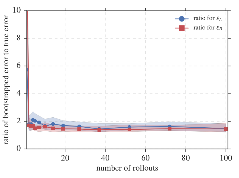
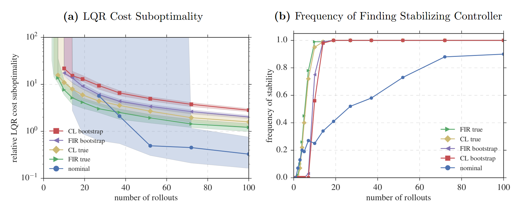
We consider a stylized temperature regulation example
\(A_\star = \begin{bmatrix} 1.01 & 0.01 & 0 \\ 0.01 & 1.01 & 0.01 \\ 0 & 0.01 & 1.01\end{bmatrix}, ~~B_\star = I\)
with relatively low penalty on state
\(Q=10^{-3}\cdot I, ~~R = I\)
What is interesting about LQR?
Nonlinear system identification and control are both much more challenging, and many strategies use LQR as a building block (iLQR, MPC).
Mania, Tu, Recht. "Certainty Equivalence is Efficient for Linear Quadratic Control." NeuRIPS, 2019.
Simchowitz, Mania, Tu, Jordan, Recht. "Learning without mixing: Towards a sharp analysis of linear system identification." COLT, 2018.
For details, see our paper: "On the sample complexity of the linear quadratic regulator." Foundations of Computational Mathematics (2019): 1-47.
By Sarah Dean


