


Sarah Dean PRO
asst prof in CS at Cornell
(down arrow to see handout slides)
| Dimension (\(d\)) | Edge Length (\(\ell\)) |
|---|---|
| 2 | 0.1 |
| 10 | 0.63 |
| 100 | 0.955 |
| 1000 | 0.9954 |
For \(k=10, n=1000\)
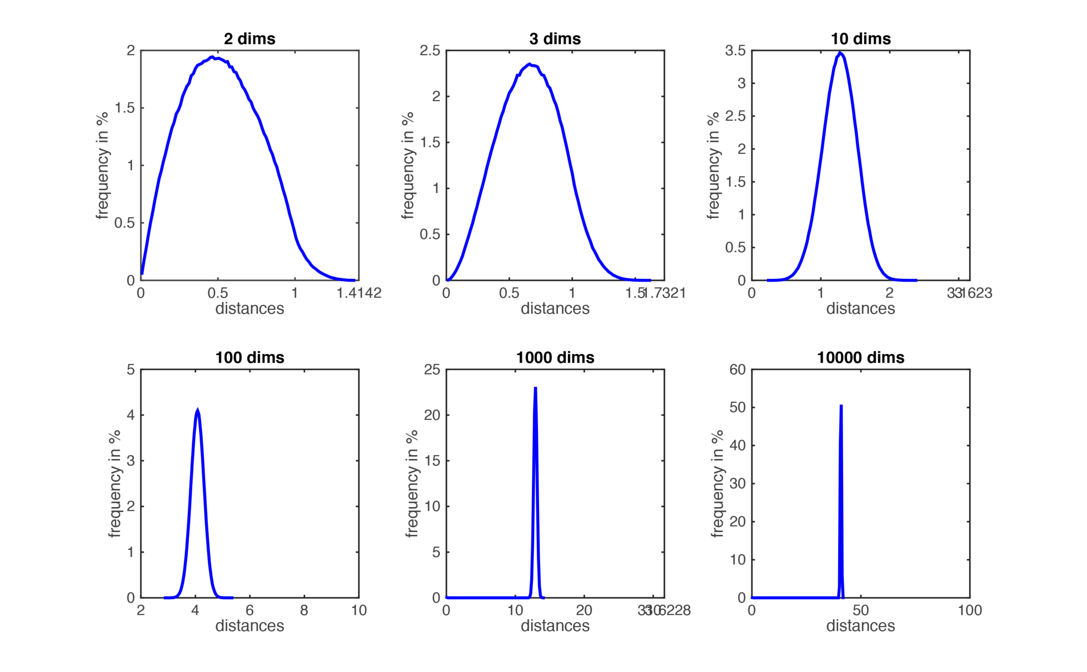
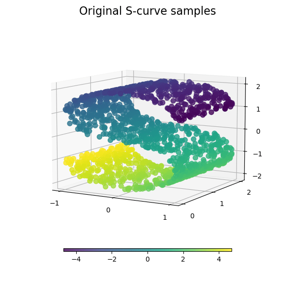
The distributions of all pairwise distances between randomly distributed points within \(d\)-dimensional unit squares.
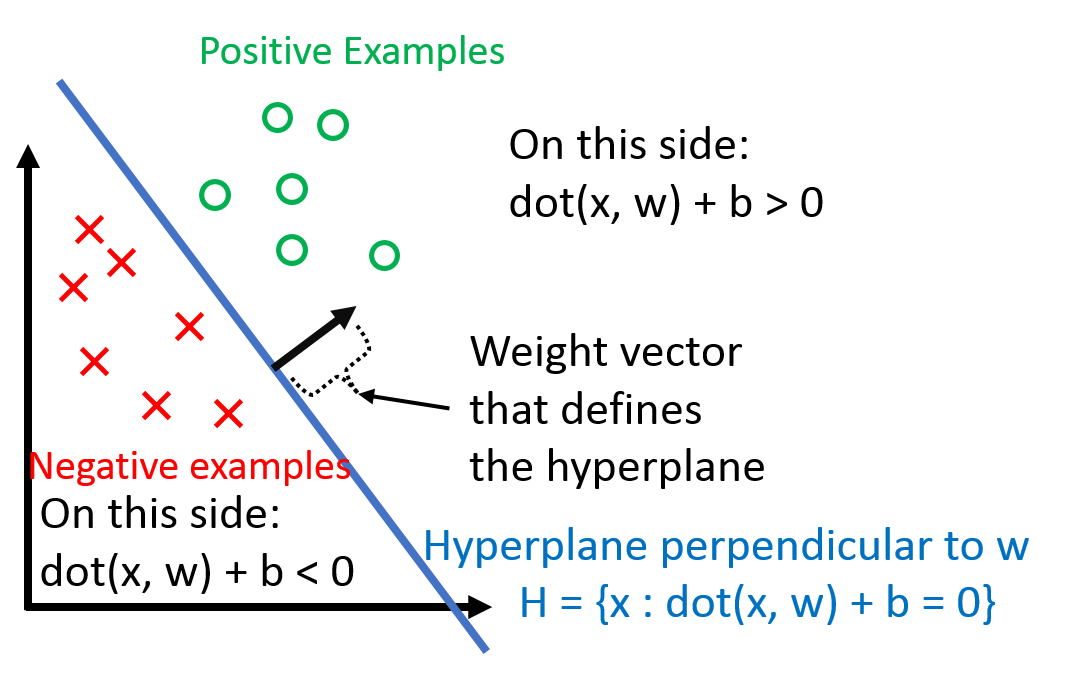
$$ h(\mathbf{x}_i) = \textrm{sign}(\mathbf{w}^\top \mathbf{x}_i + b) $$
hyperplane: \(\mathbf{w}^\top \mathbf{x}_i + b =0\)
\(\bf w\)
\(0\)
\(\underbrace{\qquad\quad}_{-b}\)
\(\bf x\)
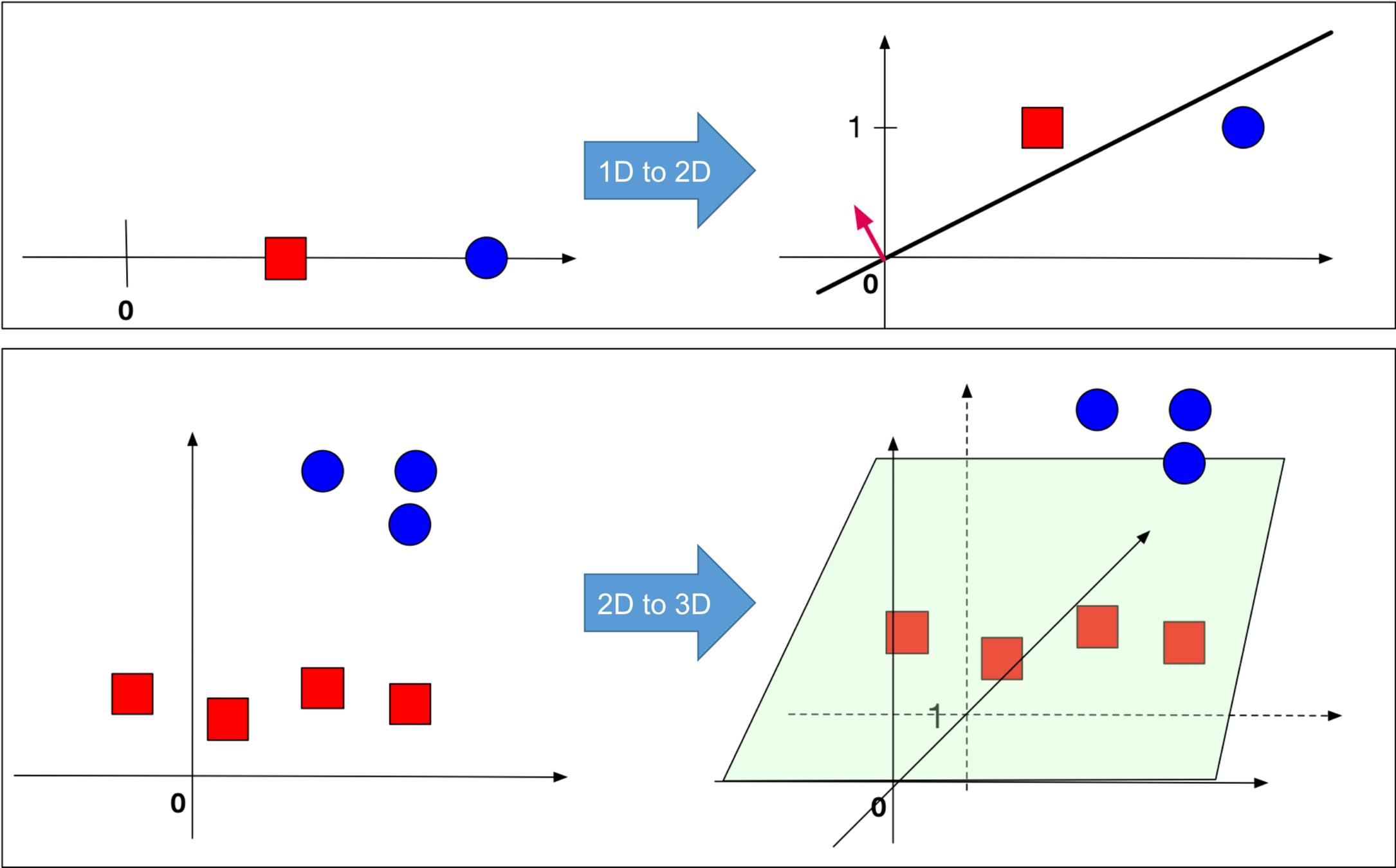
$$ \mathbf{x}_i \hspace{0.1in} \rightarrow \hspace{0.1in} \begin{bmatrix} \mathbf{x}_i \\ 1 \end{bmatrix},\qquad \mathbf{w} \hspace{0.1in} \rightarrow \hspace{0.1in} \begin{bmatrix} \mathbf{w} \\ b \end{bmatrix} $$
Initialize: \(\mathbf{w} = \mathbf{0}\)
While TRUE:
1 2 3
4 5 6
7 8 9
1 2 3
4 5 6
7 8 9
1 2 3
4 5 6
7 8 9
1 2 3
4 5 6
7 8 9
1 2 3
4 5 6
7 8 9
Form a group of \(d=9\)
Each group member tracks a weight!
\(\bf x_1=\)
\(\bf x_2=\)
\(y_1=+1\)
\(y_2=-1\)
1 2 3
4 5 6
7 8 9
Input: Training data \(D = \{(\mathbf{x}_1, y_1), ..., (\mathbf{x}_n, y_n)\}\)
Initialize: \(\mathbf{w} = \mathbf{0}\)
While TRUE:
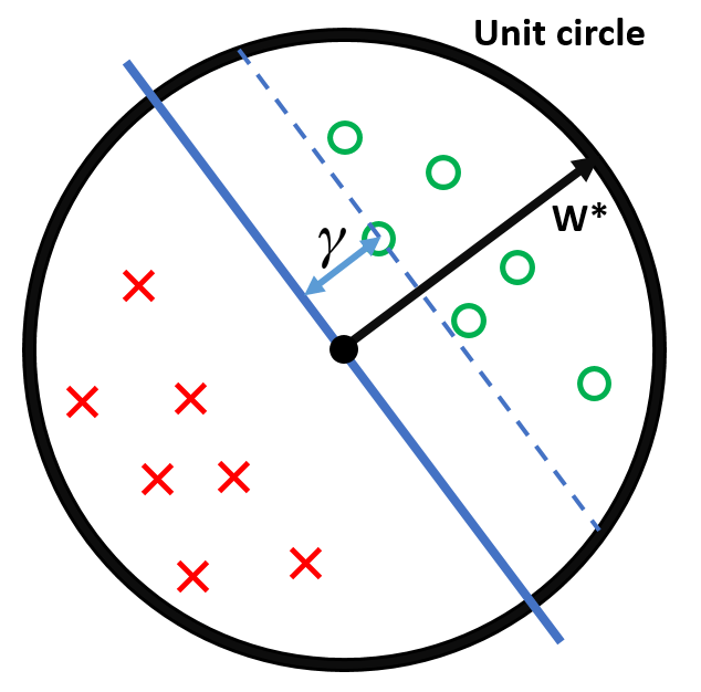
Setup: \(\|\mathbf{w}^*\| = 1\), \(\|\mathbf{x}_i\| \le 1~~\forall~ \mathbf{x}_i \in D\),
margin \( \gamma = \min_{(\mathbf{x}_i, y_i) \in D}|\mathbf{x}_i^\top \mathbf{w}^* | \)
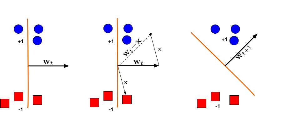
1. hyperplane misclassifies one red (-1) and one blue (+1) point
2. \(\bf x\) is chosen and used for an update.
3. updated hyperplane separates the two classes
x
x
o
o
\(\bf w\)
\(\bf w\)
\(1\)
\(\vec v\)
\(\vec u\)
)
\(\theta\)
\(\vec v\)
\(\vec u\)
\(\vec u \cdot \vec v=0\)
\(\vec u \cdot \vec v>0\)
\(\vec u \cdot \vec v<0\)
\(\vec v\)
\(\vec u\)
)
This means that for each update, \(\mathbf{w}^\top \mathbf{w}^* \) grows by at least \(\gamma\) and \(\mathbf{w}^\top \mathbf{w}\) grows by at most 1.
After \(M\) updates, (1) \(\mathbf{w}^\top\mathbf{w}^*\geq M\gamma\) and (2) \(\mathbf{w}^\top \mathbf{w}\leq M\)
Starting with (1) and ending with (2) $$ \begin{align*} M\gamma &\le \mathbf{w}^\top \mathbf{w}^* \\ &=\|\mathbf{w}\|\|\mathbf{w}^*\|\cos(\theta) \\ &\leq \|\mathbf{w}\| \\ &= \sqrt{\mathbf{w}^\top \mathbf{w}} \le \sqrt{M} \end{align*} $$
Rearranging \(M\gamma \le \sqrt{M}\), we conclude \(M \le {1}/{\gamma^2}\)
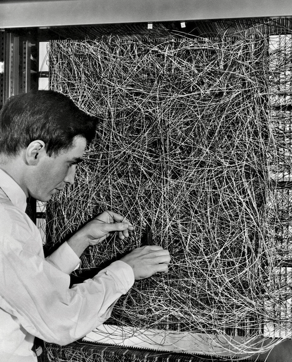
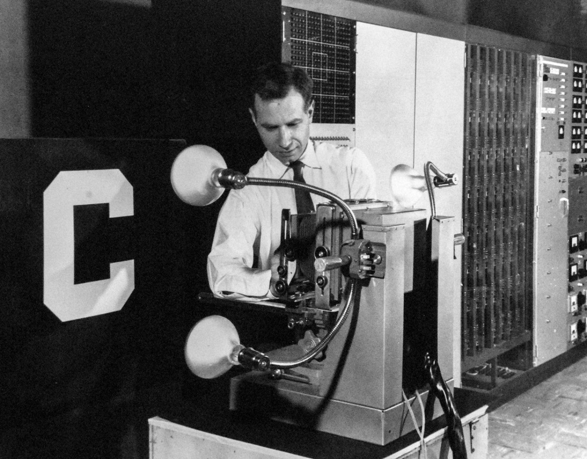
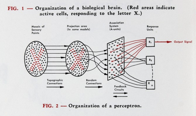
Frank Rosenblatt
New York Times, 1958
IBM 704
MARK I
Perceptron, 1960
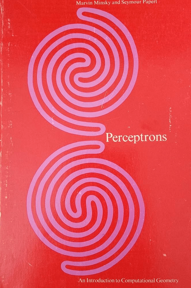
Minsky & Papert
Perceptrons, 1969
\(\underbrace{\quad\qquad\qquad}_{\vec x}\)
\(\underbrace{\qquad}_{h_{\vec w}}\)
\({\vec w}\)
\(\underbrace{\qquad}\)
updates
with \(\vec y\)
\(\underbrace{\qquad}\)
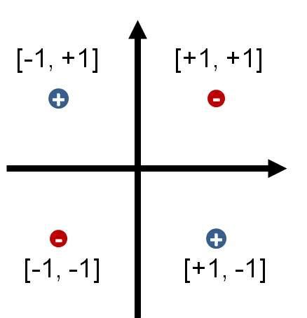
No good algorithm for multiple layers (yet)
Fundamental limitations of linear classifiers (XOR)
By Sarah Dean


