Large-scale models and simulation methods for transportation
Sebastian Hörl
6 September 2023
Spring 2024
Université Gustave Eiffel
IRT SystemX
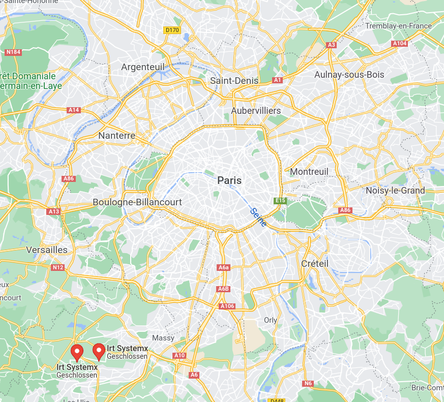
- Research foundation situated in Paris (Saclay Campus)
- Focus on fostering digital transition in a range of fields from transport, health, cybersecurity to circular economy
- Transferring research results and tools into active application by development and provision of industry platforms
- Various collaborative projects with multiple French companies (Renault, SNCF, ...) and academic partners (Université Paris Saclay, CentraleSupélec, Université Gustave Eiffel)
- Participation in European projects
Context
- We are facing climate change and transport is one of the largest contributors


Context
- We are facing climate change and transport is one of the largest contributors
- However, we need transport to
- Move people
- Move goods
Context
- We are facing climate change and transport is one of the largest contributors
- However, we need transport to
- Move people
- Move goods
- Various options:
- Move less!
Context
- We are facing climate change and transport is one of the largest contributors
- However, we need transport to
- Move people
- Move goods
- Various options:
- Move less!
- Reduce impact (electric, hydrogen, ...)
Context
- We are facing climate change and transport is one of the largest contributors
- However, we need transport to
- Move people
- Move goods
- Various options:
- Move less!
- Reduce impact (electric, hydrogen, ...)
- Become more efficient
Context
- Traditionally, transport planning asked where to build new highways or metro lines
- Nowadays, the question becomes how to use our infrastructure more efficiently, enabled by digital technology and connectivity
- On-demand transport may be a solution
- Avoid cars standing around 90% of the day
- Make efficient use of resources
- Provide access to formerly decoupled areas
- Replace half-utilized bus lines
- ...
- To understand these systems, we need highly dynamic models and simulations; and fortunately, data is become more and more available!
Goals of this course
-
Goal I: Learn where to find and how to work with large-scale open data in France
-
Goal II: Familiarize yourself with a range of data processing tools from data science, modelling, visualization and mapping
-
Goal III: Get to know modern research and planning tools from agent-based simulation
- Goal IV: Gain basic knowledge in transport planning and how to set up transport models, from raw data to the final model


Topics and tools
- To follow along in the exercises in the final project, you'll need to install a couple of tools
- A working Python environment with Jupyter (ideally conda-based)
- with the following packages
- A working Python environment with Jupyter (ideally conda-based)


Topics and tools
- Later on in the course you will need to install some additional tools for Java
- A working Java IDE like one of the following
- so that we can run
- A working Java IDE like one of the following


IntelliJ
VSCode
Topics and tools
- Finally, for mapping purposes, you may install QGIS

Data
- We will work with various data sets in the exercises
- Some of them are rather large, so it will make sense to download them beforehand!
- Links can be found in the


Agenda and course structure
18 January
19 January
23 January
25 January
8 February
10h45 CM
Trip generation & distribution
14h00 TD
Working with transport data
14h00 CM
Mode choice & Traffic assignment
16h15 TD
Modeling with transport data
14h00 CM
Synthetic populations and demand
16h15 TD
Working with synthetic demand data
14h00 CM
Agent-based transport simulation
16h15 TD
Working with MATSim
14h00 CM
On-demand service simulation
16h15 TD
On-demand service simulation
31 March
Submission of course project
- The exercises are structured so you can code along
- Make sure to attend with your personal computer or in groups with at least one machine
- The course material can be found online
Agenda and course structure
18 January
19 January
23 January
25 January
8 February
10h45 CM
Trip generation & distribution
14h00 TD
Working with transport data
14h00 CM
Mode choice & Traffic assignment
16h15 TD
Modeling with transport data
14h00 CM
Synthetic populations and demand
16h15 TD
Working with synthetic demand data
14h00 CM
Agent-based transport simulation
16h15 TD
Working with MATSim
14h00 CM
Q&A
16h15 TD
Q&A
31 March
Submission of course project
- The exercises are structured so you can code along
- Make sure to attend with your personal computer or in groups with at least one machine
- The course material can be found online
Course project
- The goal of the course project is to show how to set up a (siplified) transport model from scratch, starting with raw data
- You will work on a territory of your choice to set up your own model
- Exploring the territory through a basic data analysis
- Generating the travel demand for the study area
- Performing an agent-based simulation of an on-demand mobility service
- All instructions can be found at the link on the right
- You may start working on your project right after the first TD and you will obtain the knowledge for each exercise on the way through the course
- A report has to be handed in by 31 March 2024
- You may work in groups of up to 4 persons

1.1 Four-step model
Four-step model
- Goal: Analyse how changes in demand, habits, offers, and infrastructure impact the use of the transport system
- Model in four steps that answer four questions:
- Where do travellers come from?
- Where do they go to?
- How do they perform these trips (transport modes)?
- How heavily are services and infrastructure utilized?
Trip generation
Trip distribution
Mode choice
Traffic assignment
Four-step model
-
Question: Where do travellers come from?
-
Goal: Obtain a number of originating trips for a number of zones defined in the study area
- Number of generated trips may depend on the total population, the age distribution in a zone, the distribution of job types, ...
- Usually focus on the morning peak hour
- "How many people go to work at around 8pm?"
- Sometimes also evening peak, midday offpeak, evening off-peak
- Modelling task: Set up a model that yields the number of originating trips at a certain time given specific inputs per origin zone
Trip generation
Trip distribution
Mode choice
Traffic assignment
Four-step model
-
Question: Where do the generated travellers go to?
-
Goal: Obtain a matrix of movements between all zones (origins) to all other zones (destinations)
- Flows between two zones may be affected by
- how well the two zones are connected
- how attractive it is to go to another zone
- For instance, often, the amount and quality of employment in a zone determines if the zone is attractive for commuters
- Modelling task: Set up a model that takes into account characteristics of an origin zone, a destination zone, how well they are connected and which yields the expected flow between these zones.
Trip generation
Trip distribution
Mode choice
Traffic assignment
Four-step model
-
Question: How do people go from one zone to another?
-
Goal: Understand how people decide which mode of transport (and which route) they choose to go from A to B
- Mode choice is heavily impacted by
- travel time
- monetary cost
- number of transfers (public transport)
- waiting time (public transport, on-demand transport)
- ...
- Modelling task: Set up a model, which, given a set of alternative ways of going from A to B with their characteristics, yield the probability of either alternative being chosen.
Trip generation
Trip distribution
Mode choice
Traffic assignment
Four-step model
-
Question: How is the infrastructure impacted by travel decisions?
-
Goal: Find out how many cars make use of the road network or how many travellers the public transport services and how much time it takes to travel
- The last modelling step helps to understand if changes in generation, distribution or mode choice lead to saturation of the system
- Modelling task: Set up a model that determines which roads and transit lines will be used by the travellers and yields the travel times
Trip generation
Trip distribution
Mode choice
Traffic assignment
Four-step model
- It is possible to run the model in an iterative way:
- Accessibility of a zone may impact how likely people are to live there (generation)
- Travel times between two zones may impact how likely people are to work in a specific area (distribution)
- Travel times between two zones may impact which modes of transport people use to move between them (mode choice)
- Accessibility of a zone may impact how likely people are to live there (generation)
- In such a setting, the model is run in a feedback loop until key indicators (travel times, flows, ...) stabilize, demand and supply go then into equilibrium
Trip generation
Trip distribution
Mode choice
Traffic assignment
1.2 Trip generation
Trip generation
O_{i} = f(X_i)
- Modelling task: Set up a model that yields the number of originating trips at a certain time given specific inputs per origin zone
Trip generation
Trip distribution
Mode choice
Traffic assignment
Trip generation
O_{i} = f(X_i)
- Modelling task: Set up a model that yields the number of originating trips at a certain time given specific inputs per origin zone
Trip generation
Trip distribution
Mode choice
Traffic assignment
Characteristics of zone i
Trip generation
O_{i} = f(X_i)
- Modelling task: Set up a model that yields the number of originating trips at a certain time given specific inputs per origin zone
Trip generation
Trip distribution
Mode choice
Traffic assignment
Characteristics of zone i
Model
Trip generation
O_{i} = f(X_i)
- Modelling task: Set up a model that yields the number of originating trips at a certain time given specific inputs per origin zone
Trip generation
Trip distribution
Mode choice
Traffic assignment
Generated trips for zone i
Characteristics of zone i
Model
Trip generation
- Example: Growth factor model
- More complex models (ML, DL, ...) exist
- First approach:
Trip generation
Trip distribution
Mode choice
Traffic assignment
O_{i} = f(n_i|\beta) = \beta \cdot n_i
Trip generation
- Example: Growth factor model
- More complex models (ML, DL, ...) exist
- First approach:
Trip generation
Trip distribution
Mode choice
Traffic assignment
Population in zone i
O_{i} = f(n_i|\beta) = \beta \cdot n_i
Trip generation
- Example: Growth factor model
- More complex models (ML, DL, ...) exist
- First approach:
Trip generation
Trip distribution
Mode choice
Traffic assignment
Population in zone i
Growth factor
O_{i} = f(n_i|\beta) = \beta \cdot n_i
Trip generation
- Example: Growth factor model
- More complex models (ML, DL, ...) exist
- First approach:
- How do we estimate the parameter?
Trip generation
Trip distribution
Mode choice
Traffic assignment
Population in zone i
Growth factor
\text{min}_\beta \sum_i (f(X_i|\beta) - \hat O_i)^2
O_{i} = f(n_i|\beta) = \beta \cdot n_i
Reference value
Trip generation
- Example: Growth factor model
- More complex models (ML, DL, ...) exist
- First approach:
- How do we estimate the parameter?
Trip generation
Trip distribution
Mode choice
Traffic assignment
Population in zone i
Growth factor
\text{min}_\beta \sum_i (f(X_i|\beta) - \hat O_i)^2
O_{i} = f(n_i|\beta) = \beta \cdot n_i
Linear regression
Ordinary least squares
Trip generation
- Example: Growth factor model
- More complex models (ML, DL, ...) exist
- First approach:
- How do we estimate the parameter?
Trip generation
Trip distribution
Mode choice
Traffic assignment
Population in zone i
Growth factor
\text{min}_\beta \sum_i (f(X_i|\beta) - \hat O_i)^2
O_{i} = f(n_i|\beta) = \beta \cdot n_i
Linear regression
Ordinary least squares
\beta = \frac{\sum_i \hat O_i n_i}{\sum_i n_i^2}
Trip generation
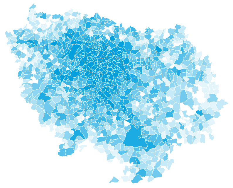
- Let's test our model!
Population in Île-de-France by municipality
n_i
O_{i} = f(n_i|\beta) = \beta \cdot n_i
Source: INSEE RP
\hat O_i
Commuters in Île-de-France
Source: INSEE RP
Source: INSEE MOBPRO
12,262,544
5,420,092


Trip generation
- Let's test our model!
Population in Île-de-France by municipality
n_i
O_{i} = f(n_i|\beta) = \beta \cdot n_i
Source: INSEE RP
Source: INSEE RP
\beta = \frac{\sum_i \hat O_i n_i}{\sum_i n_i^2} = 0.4552
12,262,544
5,420,092
\hat O_i
Commuters in Île-de-France
Source: INSEE MOBPRO
Trip generation
- Let's test our model!
Population in Île-de-France by municipality
n_i
O_{i} = f(n_i|\beta) = \beta \cdot n_i
Source: INSEE RP
Source: INSEE RP
O_i
Model results
12,262,544
5,420,092

\hat O_i
Commuters in Île-de-France
Source: INSEE MOBPRO
Trip generation
- Let's test our model!
Population in Île-de-France by municipality
n_i
O_{i} = f(n_i|\beta) = \beta \cdot n_i
Source: INSEE RP
Source: INSEE RP
Difference

O_i - \hat O_i
\hat O_i
Commuters in Île-de-France
Source: INSEE MOBPRO
12,262,544
5,420,092
Trip generation
- Let's test our model!
Population in Île-de-France by municipality
n_i
O_{i} = f(n_i|\beta) = \beta \cdot n_i
Source: INSEE RP
Source: INSEE RP
\hat O_i
Commuters in Île-de-France
Source: INSEE MOBPRO

12,262,544
5,420,092
Trip generation
- Let's test our model!
Population in Île-de-France by municipality
n_i
O_{i} = f(n_i|\beta) = \beta \cdot n_i
Source: INSEE RP
Source: INSEE RP
\hat O_i
Commuters in Île-de-France
Source: INSEE MOBPRO
Are we happy with this model?
12,262,544
5,420,092
Trip generation
- Next try:
O_{i} = f(n_i|\beta) = \beta_0 + \sum_s \beta_s \cdot n_{is}

Source: INSEE
Population by socio-professional category in Île-de-France
CSP = Catégorie socio-professionelle
The socio-professional category is a common statistical tool in France to perform analyses based on different employment levels in France with eight categories
Trip generation
- Next try:
Population by CSP
Source: INSEE
Population by socio-professional category in Île-de-France
CSP = Catégorie socio-professionelle
The socio-professional category is a common statistical tool in France to perform analyses based on different employment levels in France with eight categories
O_{i} = f(n_i|\beta) = \beta_0 + \sum_s \beta_s \cdot n_{is}
Trip generation
Growth factor by CSP
Source: INSEE
Population by socio-professional category in Île-de-France
CSP = Catégorie socio-professionelle
The socio-professional category is a common statistical tool in France to perform analyses based on different employment levels in France with eight categories
- Next try:
Population by CSP
O_{i} = f(n_i|\beta) = \beta_0 + \sum_s \beta_s \cdot n_{is}
Trip generation
- Let's test our model!
Intellectual professions (CSP 3)
Workers (CSP 6)
O_{i} = f(n_i|\beta) = \beta_0 + \sum_s \beta_s \cdot n_{is}
Employees (CSP 5)


Trip generation
- Let's test our model!
CSP Model
\hat O_i
Commuters in Île-de-France
Source: INSEE MOBPRO
Simple model

O_{i} = f(n_i|\beta) = \beta_0 + \sum_s \beta_s \cdot n_{is}
Trip generation
- Let's test our model!
\hat O_i
Commuters in Île-de-France
Source: INSEE MOBPRO
CSP Model

O_{i} = f(n_i|\beta) = \beta_0 + \sum_s \beta_s \cdot n_{is}
Trip generation
- We can now, for instance, apply the data on a smaller zoning system if we know the number of people in a certain CSP living there

Trip generation
- Note on trip attraction models
- The models presented here can also be used to estimate the number of trips arriving in a zone.
1.3 Trip distribution
Trip distribution
F_{ij} = f(X_i, X_j)
- Modelling task: Set up a model that takes into account characteristics of an origin zone, a destination zone, how well they are connected and which yields the expected flow between these zones.
Trip generation
Trip distribution
Mode choice
Traffic assignment
Trip distribution
F_{ij} = f(X_i, X_j)
- Modelling task: Set up a model that takes into account characteristics of an origin zone, a destination zone, how well they are connected and which yields the expected flow between these zones.
Trip generation
Trip distribution
Mode choice
Traffic assignment
Origin characteristics
Trip distribution
F_{ij} = f(X_i, X_j)
- Modelling task: Set up a model that takes into account characteristics of an origin zone, a destination zone, how well they are connected and which yields the expected flow between these zones.
Trip generation
Trip distribution
Mode choice
Traffic assignment
Destination characteristics
Model
Flow
Origin characteristics
Trip distribution
F_{ij} = f(X_i, X_j)
-
Modelling task: Set up a model that takes into account characteristics of an origin zone, a destination zone, how well they are connected and which yields the expected flow between these zones.
- Flow models are mainly concerned with large flows, for instance, commuters going to work in the peak hour
Trip generation
Trip distribution
Mode choice
Traffic assignment
Destination characteristics
Model
Flow
Origin characteristics
Trip distribution
- We can imagine F as a matrix where rows indicate the origins and columns the destinations
- Row sums are the outflows of the origin zones
- Column sums are the inflows of the destination zones

Trip distribution
- We can imagine F as a matrix where rows indicate the origins and columns the destinations
- Row sums are the outflows of the origin zones
- Column sums are the inflows of the destination zones
- Let's define
O_i = \sum_j F_{ij}
D_i = \sum_i F_{ij}
Outflow / Origins
Inflow / Destinations
Trip distribution
- We can imagine F as a matrix where rows indicate the origins and columns the destinations
- Row sums are the outflows of the origin zones
- Column sums are the inflows of the destination zones
- Let's define
- We may use a trip generation model to generate the row sums, and we may use a trip attraction model to generation the column sums
O_i = \sum_j F_{ij}
D_i = \sum_i F_{ij}
Outflow / Origins
Inflow / Destinations
Trip distribution
- Example: Zonal flows in Île-de-France
- 1,287 municipalities in total
- 1,656,369 combinations
- 123,787 combinations are available (7.4%)
Source: INSEE MOBPRO
Paris 13e
Alfortville
Melun


Trip distribution
F_{ij} = P(X_i) \cdot A(X_j) \cdot \rho(X_i, X_j)
- Gravity model: The most commonly used model is the Gravity model with the following form:
Trip distribution
F_{ij} = P(X_i) \cdot A(X_j) \cdot \rho(X_i, X_j)
- Gravity model: The most commonly used model is the Gravity model with the following form:
Production term
Trip distribution
F_{ij} = P(X_i) \cdot A(X_j) \cdot \rho(X_i, X_j)
- Gravity model: The most commonly used model is the Gravity model with the following form:
Production term
Attraction term
Trip distribution
F_{ij} = P(X_i) \cdot A(X_j) \cdot \rho(X_i, X_j)
- Gravity model: The most commonly used model is the Gravity model with the following form:
Production term
Attraction term
Friction / Resistance term
Trip distribution
F_{ij} = P(X_i) \cdot A(X_j) \cdot \rho(X_i, X_j)
-
Gravity model: The most commonly used model is the Gravity model with the following form:
Production term
Attraction term
Friction / Resistance term
- Production term: Weighs how much trips are produced by a zone
- Attraction term: Weighs how attractive a zone is for a trip to arrive
- Friction term: Quantifies how are it is to get from one zone to another (road, transit, natural obstacles, ...)
Trip distribution
F_{ij} = P(X_i) \cdot A(X_j) \cdot \rho(X_i, X_j)
-
Gravity model: The most commonly used model is the Gravity model with the following form:
- The friction term is often estimated stand-alone and upfront
- Simple approach: Friction depends on the distance between two zones
Trip distribution
F_{ij} = P(X_i) \cdot A(X_j) \cdot \rho(X_i, X_j)
-
Gravity model: The most commonly used model is the Gravity model with the following form:
- The friction term is often estimated stand-alone and upfront
- Simple approach: Friction depends on the distance between two zones
The probability of observing a commute between two municipalities in Île-de-France decreases exponentially with the distance between these municipalities
\rho_{ij} = \exp({\alpha + \beta \cdot d_{ij}})
\alpha = -0.9
\beta = 0.11

Trip distribution
F_{ij} = P(X_i) \cdot A(X_j) \cdot \rho(X_i, X_j)
-
Gravity model: The most commonly used model is the Gravity model with the following form:
- The friction term is often estimated stand-alone and upfront
- Simple approach: Friction depends on the distance between two zones
- More complex friction terms are possible and are widely used
- Travel time
- Monetary cost
- Others
Trip distribution
F_{ij} = P(X_i) \cdot A(X_j) \cdot \rho(X_i, X_j)
-
Gravity model: The most commonly used model is the Gravity model with the following form:
- The use of the gravity model depends on which data is available. The single-constrained gravity model assumes that we have reference data for the outflow of certain zones.
- Combing the gravity model with
- Gives
- And
- This fixed expression for P can be inserted in the main model from above.
O_i = \sum_j F_{ij}
O_i = P(X_i) \cdot \sum_j A(X_j) \rho(X_i, X_j)
P(X_i) = \frac{O_i}{\sum_j A(X_j) \rho(X_i, X_j)}
Trip distribution
F_{ij} = O_i \cdot \frac{A(X_j) \cdot \rho(X_i, X_j)}{\sum_j A(X_j) \cdot \rho(X_i, X_j)}
- Single-constrained gravity model
- Any choice for A will now by design of the model yield the correct origin flows
Trip distribution
F_{ij} = O_i \cdot \frac{A(X_j) \cdot \rho(X_i, X_j)}{\sum_j A(X_j) \cdot \rho(X_i, X_j)}
- Single-constrained gravity model
-
Any choice for A will now by design of the model yield the corrent origin flows
- Simple example: The attraction of a zone is dependent on the employees working in that zone
A_j = w_j^\lambda
Trip distribution
F_{ij} = O_i \cdot \frac{A(X_j) \cdot \rho(X_i, X_j)}{\sum_j A(X_j) \cdot \rho(X_i, X_j)}
- Single-constrained gravity model
-
Any choice for A will now by design of the model yield the correct origin flows
- Simple example: The attraction of a zone is dependent on the employees working in that zone
A_j = w_j^\lambda
Emploiment in zone j
Model parameter
Trip distribution
F_{ij} = O_i \cdot \frac{A(X_j) \cdot \rho(X_i, X_j)}{\sum_j A(X_j) \cdot \rho(X_i, X_j)}
- Single-constrained gravity model
-
Any choice for A will now by design of the model yield the correct origin flows
- Simple example: The attraction of a zone is dependent on the employees working in that zone
- We use the friction model as defined before
A_j = w_j^\lambda
Emploiment in zone j
Model parameter
\rho_{ij} = \exp({\alpha + \beta \cdot d_{ij}})
F_{ij} = O_i \cdot \frac{w_j^\lambda \cdot \rho_{ij}}{\sum_j w_j^\lambda \cdot \rho_{ij}}
Trip distribution
- Single-constrained gravity model
- Given some reference flows on the territory, we may now fit the parameter
- Alternatively, we may have some of the destination flows as data to fit
\text{min}_\beta \sum_{ij \in \mathcal{R}} \left(\hat F_{ij} - F_{ij}(\beta) \right)^2
F_{ij} = O_i \cdot \frac{w_j^\lambda \cdot \rho_{ij}}{\sum_j w_j^\lambda \cdot \rho_{ij}}
\text{min}_\beta \sum_{j \in \mathcal{R}} \left(\hat D_{j} - \sum_i F_{ij}(\beta) \right)^2
(used in the following example)
Trip distribution
- Example: Île-de-France

Trip distribution
- Example: Île-de-France
Alfortville

Data
Model

Trip distribution
- Sometimes, we may also know the destination flows
- The inflow constraint can be integrated analogously to the origins
- This leads to the double-constrained gravity model
- The values of A and P are fully determined by the observed origin and destination flows. By design, the model produces flow matrices F that have the correct row and column sums.
- The values of A and P are obtained by evaluating the two right-mode functions iteratively until the values stabilize.
F_{ij} = \frac{O_i \cdot D_j \cdot \rho_{ij}}{(\sum_i P_i \cdot \rho_{ij}) \cdot (\sum_j A_j \cdot \rho_{ij})}
D_j = \sum_j F_{ij}
P_i = \frac{O_i}{\sum_j A_j \cdot \rho_{ij}}
A_j = \frac{D_j}{\sum_i P_i \cdot \rho_{ij}}
Trip distribution
- Example: Île-de-France
1.3 Mode choice
Mode choice
Trip generation
Trip distribution
Mode choice
Traffic assignment
P(k) = f(X_1, ..., X_K)
- Modelling task: Set up a model, which, given a set of alternative ways of going from A to B with their characteristics, yield the probability of either alternative being chosen.
Mode choice
Trip generation
Trip distribution
Mode choice
Traffic assignment
P(k) = f(X_1, ..., X_K)
- Modelling task: Set up a model, which, given a set of alternative ways of going from A to B with their characteristics, yield the probability of either alternative being chosen.
Characteristics of alternative k
Mode choice
Trip generation
Trip distribution
Mode choice
Traffic assignment
P(k) = f(X_1, ..., X_K)
- Modelling task: Set up a model, which, given a set of alternative ways of going from A to B with their characteristics, yield the probability of either alternative being chosen.
Characteristics of alternative k
Probability of choosing k
Mode choice
Trip generation
Trip distribution
Mode choice
Traffic assignment
P(k) = f(X_1, ..., X_K)
- Modelling task: Set up a model, which, given a set of alternative ways of going from A to B with their characteristics, yield the probability of either alternative being chosen.
Characteristics of alternative k
Probability of choosing k
Model
Mode choice


Mode choice
Mode choice


Mode choice
Mode choice
Mode choice
Mode choice


Mode choice
Mode choice
Mode choice
- Which option will I choose?
- Which option do people statistically choose?
Mode choice
Source: Felix Becker, Institute for Transport Planning and Systems, ETH Zurich.
- A common source for choice models is survey data
Mode choice
- A common source for choice models is survey data
- They are performed in a pivot design: Each person gets to view various combinations of values.
- Difficulty I: How to design the survey?
- How many questions are too many?
- How to cover the whole range of potential values?
- Difficulty II: Respondents
- How to ensure that the survey is representative?
- How to make sure the relevant user groups are covered?
- Difficulty III: Misbehaviour
- What if somebody always selects random options?
- What if somebody always selects the first option?
- What if answers are missing?
Mode choice
- Alternative source to Stated Preference data (SP) is Revealed Preference data (RP)
- In Revealed Preference experiments, the actual choices of the persons are tracked
- What do we observe?
- SP: Hypothetic choices of the respondents
- RP: Actual choices of the respondents
- What is known?
- SP: Full knowledge about all choices
- RP: Only knowledge about the taken choice, all alternatives need to be reconstructed!
Mode choice
- Alternative sources are data sets in which people have been asked about the trips they did during one day
- Alternatives to the chosen option need to be generated a posteriori
- Île-de-France
- Enquête Globale de Transport (EGT)
- (2010, on request); (2015 on yet published)
- Nantes, Lyon, Lille, ...
- Enquête Déplacements Grand Territoire (EDGT)
- Available for various years depending on city
- Sometimes publicly accessible as open data (Nantes, Lille)
- France
-
Enquête Nationale Transports et Déplacements (ENTD)
- From 2008, available as open data
-
Enquête Nationale Transports et Déplacements (ENTD)
Mode choice
- A common mode choice model is the multinomial logit model
- The idea is that the utility of an alternative can be quantified:
v_{ik} = \beta_{1} \cdot x_{i1} + \beta_{2} \cdot x_{i2} + ... = \sum_q \beta_q \cdot x_{iq}
Mode choice
- A common mode choice model is the multinomial logit model
- The idea is that the utility of an alternative can be quantified:
v_{ik} = \beta_{1} \cdot x_{i1} + \beta_{2} \cdot x_{i2} + ... = \sum_q \beta_q \cdot x_{iq}
Value of variable q
Mode choice
- A common mode choice model is the multinomial logit model
- The idea is that the utility of an alternative can be quantified:
v_{ik} = \beta_{1} \cdot x_{i1} + \beta_{2} \cdot x_{i2} + ... = \sum_q \beta_q \cdot x_{iq}
Influence weight of variable q
Value of variable q
Mode choice
- A common mode choice model is the multinomial logit model
- The idea is that the utility of an alternative can be quantified:
v_{ik} = \beta_{1} \cdot x_{i1} + \beta_{2} \cdot x_{i2} + ... = \sum_q \beta_q \cdot x_{iq}
Influence weight of variable q
Value of variable q
Systematic utility of alternative k for decision-maker i
Mode choice
- A common mode choice model is the multinomial logit model
- The idea is that the utility of an alternative can be quantified:
- In general, we have K alternatives, we have Q variables (or inputs, like travel time, monetary costs, number of transfers, ...), and N decision-makers (observations)
- Systematic utilities are also called generalized costs
v_{ik} = \beta_{1} \cdot x_{i1} + \beta_{2} \cdot x_{i2} + ... = \sum_q \beta_q \cdot x_{iq}
Systematic utility of alternative k for decision-maker i
Influence weight of variable q
Value of variable q
Mode choice
- A common mode choice model is the multinomial logit model
- The idea is that the utility of an alternative can be quantified:
- A rational decision-maker (homo oeconomicus) would then choose the alternative that has the highest utility!
v_{ik} = \beta_{1} \cdot x_{i1} + \beta_{2} \cdot x_{i2} + ... = \sum_q \beta_q \cdot x_{iq}
Systematic utility of alternative k for decision-maker i
Influence weight of variable q
Value of variable q
y_i = \text{arg max}_k \{ v_{i1}, ..., v_{ik}, ... v_{iK} \}
Chosen alternative
Mode choice
-
Example: Choice between two public transport connections
v_k = \beta_\text{travelTime} \cdot x_{k, \text{travelTime}} + \beta_\text{interchanges} \cdot x_{k, \text{interchanges}}
Connection A
x_{A, \text{travelTime}} = 20\ \text{min}
Connection B
x_{B, \text{travelTime}} = 30\ \text{min}
x_{B, \text{interchanges}} = 0
x_{A, \text{interchanges}} = 1
Mode choice
-
Example: Choice between two public transport connections
Connection A
x_{A, \text{travelTime}} = 20\ \text{min}
Connection B
x_{B, \text{travelTime}} = 30\ \text{min}
x_{B, \text{interchanges}} = 0
x_{A, \text{interchanges}} = 1
-0.6
-1.0
v_k = \beta_\text{travelTime} \cdot x_{k, \text{travelTime}} + \beta_\text{interchanges} \cdot x_{k, \text{interchanges}}
Mode choice
-
Example: Choice between two public transport connections
Connection A
x_{A, \text{travelTime}} = 20\ \text{min}
Connection B
x_{B, \text{travelTime}} = 30\ \text{min}
x_{B, \text{interchanges}} = 0
x_{A, \text{interchanges}} = 1
-0.6
-1.0
-0.6 * 20 - 1.0 * 1 = -13
-0.6 * 30 - 1.0 * 0 = -19
v_k = \beta_\text{travelTime} \cdot x_{k, \text{travelTime}} + \beta_\text{interchanges} \cdot x_{k, \text{interchanges}}
Mode choice
- In vector form, the utility maximization model can be written as:
- To find the correct parameters, would need:
- N observations of decisions taken
- Each observation states a chosen alternative
- Each observation states the respective choice characteristics
- The task is then:
v_k(X_i) = \beta_k^T \cdot X_i
Find
\beta^*
such that
y_i = \text{arg max}_k \{ v_k(X_i\ |\ \beta^*) \} \ \
\forall i
!
Mode choice
- In vector form, the utility maximization model can be written as:
- To find the correct parameters, would need:
- N observations of decisions taken
- Each observation states a chosen alternative
- Each observation states the respective choice characteristics
- The task is then:
v_k(X_i) = \beta_k^T \cdot X_i
Find
\beta^*
such that
y_i = \text{arg max}_k \{ v_k(X_i\ |\ \beta^*) \} \ \
\forall i
Parameters we want to find
Characteristics of all alternatives
Systematic utility per alternative
Actual choice taken by the person
!
No exact solution can exist!
Mode choice
-
Idea: No exact solution exists, because human decisions are partly random. What if we introduce randomness into our model?
- Based on our systematic utility, we introduce a random utility
- We have added an independent random error term over all alternatives for all decision-makers
- A straightforward choice would be to use a Normal distribution
- Mathematically, we still select the best alternative, but is this better?
- In any case, we call this a Random Utility Model (RUM)
u_{ik} = v_{ik} + \sigma \epsilon_{ki}
\text{E}[\epsilon_{ik}] = 0
\sigma \geq 0
with
y_i = \text{arg max}_k \{ v_k(X_i\ |\ \beta^*) + \sigma \epsilon_{ik} \} \ \
\forall i
Mode choice
- Is it better? Yes, but we need a special case!
- A straightforward expression can be obtained if we use an Extreme Value Distribution like the Gumbel Distribution
- Then it has been shown that there is a correspondance between:
\epsilon_{ik} \sim EV
(Lots of math)
[Daniel McFadden in the 70s]
u_{ik} = v_{ik} + \sigma \epsilon_{ki}
y_i = \text{arg max}_k \{ u_{ik} \}
P[y_i] = \frac{\exp\left(\sigma^{-1}v_k\right)}{\sum_{k'}\exp\left(\sigma^{-1}v_{k'}\right)}
Mode choice
- With this finding, discrete choice modeling has been revolutionized in the 70s
- The expression on the right is now a closed-form expression of the probability of choosing alternative y
- The model is called the Multinomial Logit Model. It is the most commonly used approach for choice modelling today (with a large variety of extensions and versions).
- Why has it been so impactful? Because it allows us to estimate the model parameters that are hidden in the systematic utility v in the equation above.
u_{ik} = v_{ik} + \sigma \epsilon_{ki}
P[y_i] = \frac{\exp\left(\sigma^{-1}v_k(X_i|\beta)\right)}{\sum_{k'}\exp\left(\sigma^{-1}v_{k'}(X_i|\beta)\right)}
Mode choice
- Having a closed-form expression allows us to perform a Maximum Likelihood Estimation (MLE) of the model parameters. For that we set up the likelihood function of the model:
- It answers: How well does the model (with given parameters) explain the choices?
- The maximum likelihood estimate for the model parameters is then:
- It can be found using standard methods such as Gradient Descent or Newton-Raphson
u_{ik} = v_{ik} + \sigma \epsilon_{ki}
\pi[y_i|\beta] = \frac{\exp\left(\sigma^{-1}v_k(X_i|\beta)\right)}{\sum_{k'}\exp\left(\sigma^{-1}v_{k'}(X_i|\beta)\right)}
\mathcal{L}(\beta|y_{1:N}) = \prod_i \pi(y_i | \beta)
\mathcal{l}(\beta|y_{1:N}) = \sum_i \log( \pi(y_i | \beta) )
\hat \beta_{MLE} = \argmax_{\beta} \mathcal{l}(\beta|y_{1:N})
Mode choice
-
More elaborate example
Mode choice
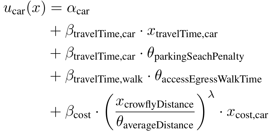
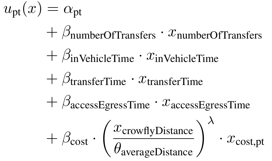
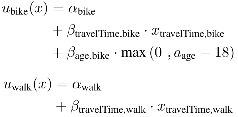
- Utility is an abstract mathematical concept. On the contrary, most choice characteristics have a unit, for instance distance, travel time, money
- Let's redefine , i.e. we transform all parameters into a new space
- With we get the Value of Travel Time Savings
v = \beta_\text{travelTime} \cdot x_\text{travelTime} \\
+ \beta_\text{cost} \cdot x_\text{cost}
[1/min] * [min]
[1/EUR] * [EUR]
\beta_u = \tilde \beta_u \cdot A
A = \beta_{cost}
\tilde \beta_\text{travelTime} = \beta_\text{travelTime} / \beta_{cost}
\tilde \beta_\text{cost} = 1
[EUR/min]
[1]
Mode choice
- The Value of Travel Time Savings (VTTS) explains how much money persons (on average) would be willing to pay extra if the travel time on a specific connection is reduced by a certain amount of time.
- Other interpretation: How uncomfortable is it to spend a certain duration in one mode of transport vs. another one? The VTTS is the higher, the more "costly" or uncomfortable it is to take a trip using this transport mode.
- VTTS are relatively stable over different surveys and countries after accounting for the respective currencies.
VTTS = \tilde \beta_\text{travelTime} = \beta_\text{travelTime} / \beta_{cost}
Mode choice


13 CHF/h
AMoD
Taxi
19 CHF/h
Conventional
Car
12 CHF/h
Public
Transport
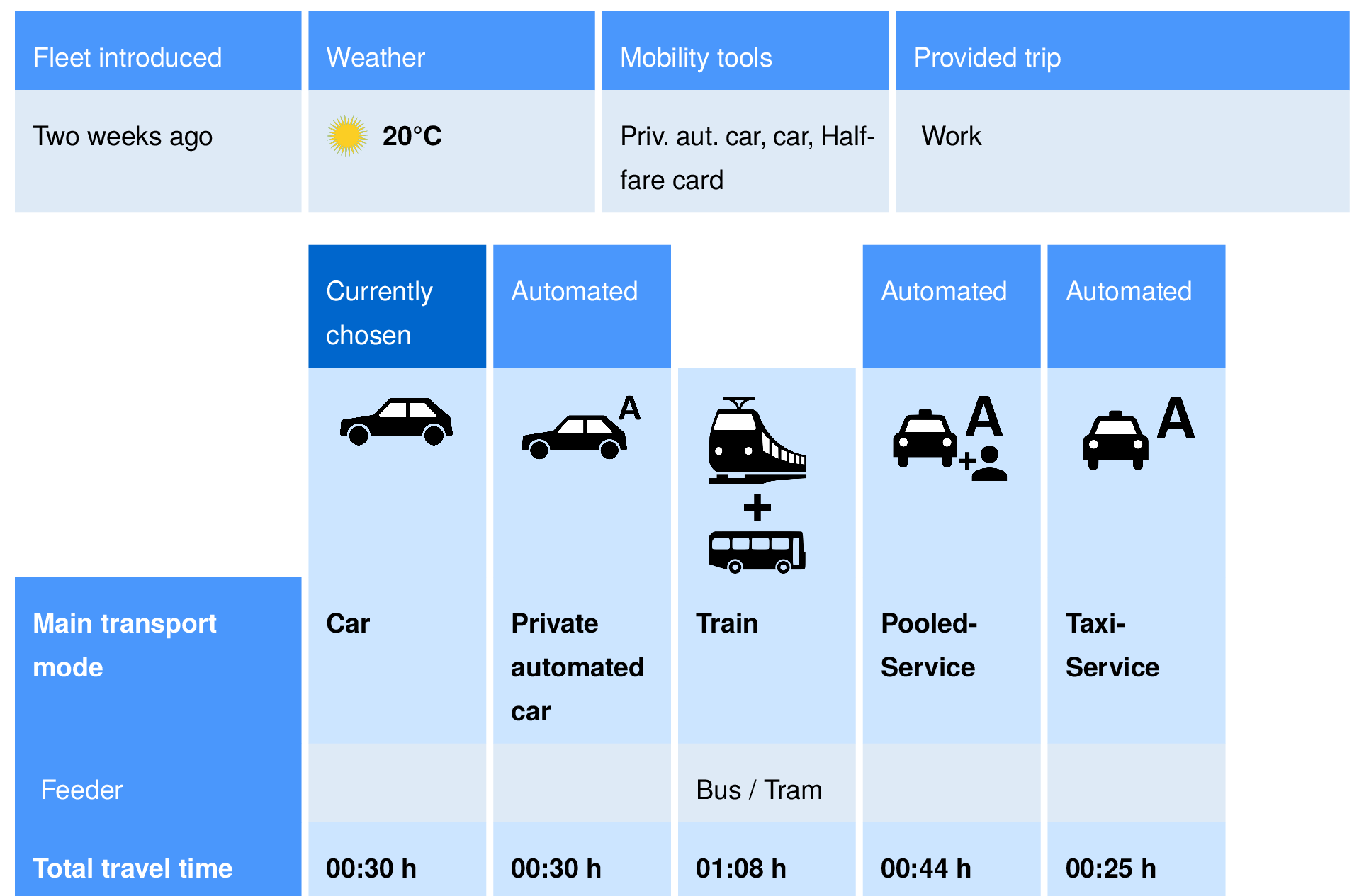
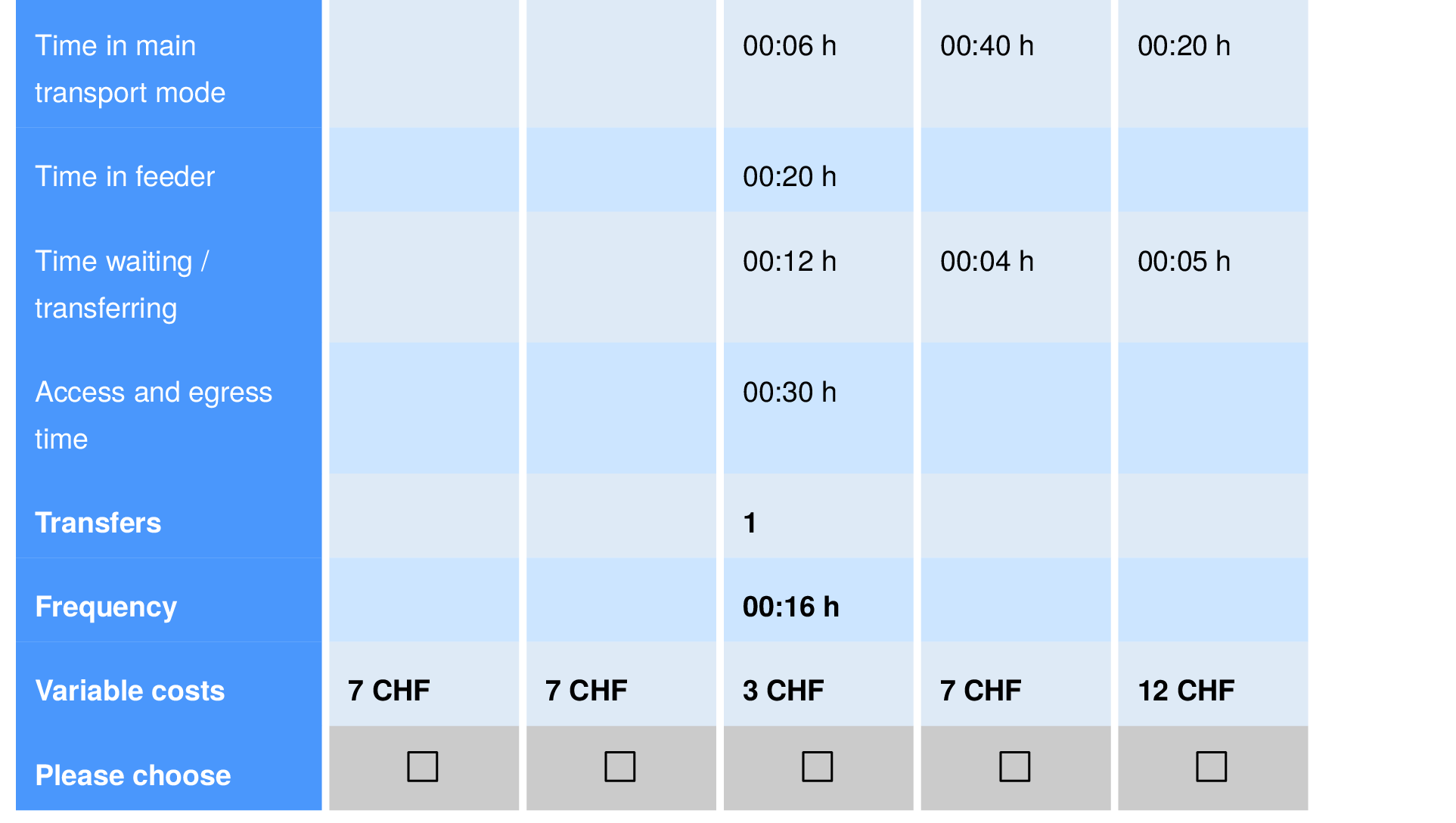
AMoD
- Remember the survey from before on the introduction of automated taxis in the transport system of Zurich?
Mode choice
13 CHF/h
AMoD
Taxi
19 CHF/h
Conventional
Car
12 CHF/h
Public
Transport
AMoD
- Remember the survey from before on the introduction of automated taxis in the transport system of Zurich?

21 CHF/h
32 CHF/h
Mode choice
13 CHF/h
AMoD
Taxi
19 CHF/h
Conventional
Car
12 CHF/h
Public
Transport
AMoD
- Remember the survey from before on the introduction of automated taxis in the transport system of Zurich?
Note on ML/DL models
- VTTS only measurable because of linear structure of the utilities
21 CHF/h
32 CHF/h
Mode choice
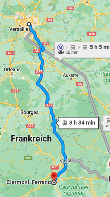
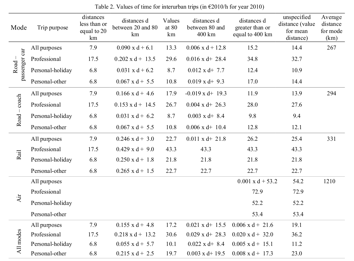
- What is the value of decreasing the travel time Paris to Clermont by 30 minutes?
- Standardized VTTS, for instance (Meunier & Quinet, 2015)
- VTTS = 21.8 EUR/h
Mode choice
- Finally, how do we use the Multinomial Logit model to make a decision for a new choice situation?
-
Option 1: Direct sampling
- Calculate systematic utilities
- Calculate probabilities
- Sample one alternative
- Calculate systematic utilities
v_k(X)
\pi_k(v_k)
y \sim \pi_k(v_k)
Mode choice
v_k(X)
\epsilon_k \sim \text{Gumbel}
y = \text{arg max}_k \left\{
v_1 + \epsilon_1, ..., v_K + \epsilon_K
\right\}
- Finally, how do we use the Multinomial Logit model to make a decision for a new choice situation?
-
Option 2: Error sampling
- Calculate systematic utilities
- Sample error terms
- Select the maximum
- Calculate systematic utilities
Mode choice
- There is a large field of discrete choice modelling with specific journals
- What happens if we replace the EV distribution by a Normal distribution?
- We get a Multinomial Probit model
- There is no analytical likelihood function any more, but simulation stays straight-forward
- Possibility to flexibly model the error term
- Correlations between choice alternatives
(if I like the red bus, I also like the blue bus)
- More complex formulations of the MNL exist
- Mainly to disentangle the above-mentioned correlation structure of errors
- Nested logit model (first I choose that I use the bus, then if I prefer red or blue)
-
Cross-nested logit model (an automated taxi is like a bus, but also a bit like a car)
- Multiplicative error terms ...
- Parameters (β) are not static but follow a distribution themselves ...
1.4 Traffic assignment
Traffic assignment
Trip generation
Trip distribution
Mode choice
Traffic assignment
X(a) = f(Q_{rs})
- Modelling task: Set up a model that determines which roads and transit lines will be used by the travellers and yields the travel times
T(a) = f(Q_{rs})
Traffic assignment
Trip generation
Trip distribution
Mode choice
Traffic assignment
X(a) = f(Q_{rs})
- Modelling task: Set up a model that determines which roads and transit lines will be used by the travellers and yields the travel times
Movements from zone r to zone s
T(a) = f(Q_{rs})
Traffic assignment
Trip generation
Trip distribution
Mode choice
Traffic assignment
X(a) = f(Q_{rs})
- Modelling task: Set up a model that determines which roads and transit lines will be used by the travellers and yields the travel times
Movements from zone r to zone s
T(a) = f(Q_{rs})
Travel times on road a
Traffic assignment
Trip generation
Trip distribution
Mode choice
Traffic assignment
X(a) = f(Q_{rs})
- Modelling task: Set up a model that determines which roads and transit lines will be used by the travellers and yields the travel times
Movements from zone r to zone s
T(a) = f(Q_{rs})
Travel times on road a
Vehicle flow on road a
Traffic assignment
Trip generation
Trip distribution
Mode choice
Traffic assignment
- Modelling task: Set up a model that determines which roads and transit lines will be used by the travellers and yields the travel times
Traffic assignment
Trip generation
Trip distribution
Mode choice
Traffic assignment
-
Modelling task: Set up a model that determines which roads and transit lines will be used by the travellers and yields the travel times
- The model is based on a rational decision maker: Individually, I will follow the route that minimizes my personal travel time.
- This is the game-theoretic Wardrop principle
- Travel times in the network are described through volume-delay functions:
T_a(x_a) = f(x_a)
Traffic assignment
-
Example: Two routes and Wardrop equilibrium
- Travel demand from S to E:
- Travel time on Route A (normal road):
- Travel time on Route B (highway):
- Travel demand from S to E:
Q_{se}=1000
t_A(x_A) = 500 + x_A \cdot 2
t_B(x_B) = 1000 + x_B \cdot 1
S
E
Route A
Route B
Traffic assignment
-
Example: Two routes and Wardrop equilibrium
- Travel demand from S to E:
- Travel time on Route A (normal road):
- Travel time on Route B (highway):
- Travel demand from S to E:
Q_{se}=1000
t_A(x_A) = 500 + x_A \cdot 2
t_B(x_B) = 1000 + x_B \cdot 1
S
E
Route A
Route B
How many cars use routes A and B and what is the travel time?
Traffic assignment
-
Example: Two routes and Wardrop equilibrium
- Travel demand from S to E:
- Travel time on Route A (normal road):
- Travel time on Route B (highway):
- Flow must be distributed over the routes:
- Wardrop: If the travel time on Route A is quicker than Route B, I would not use Route A, but rather Route B!
- Travel demand from S to E:
Q_{se}=1000
t_A(x_A) = 500 + x_A \cdot 2
t_B(x_B) = 1000 + x_B \cdot 1
S
E
Route A
Route B
x_A + x_B = Q_{se}
?
Traffic assignment
-
Example: Two routes and Wardrop equilibrium
- Travel demand from S to E:
- Travel time on Route A (normal road):
- Travel time on Route B (highway):
- Flow must be distributed over the routes:
- Wardrop: If the travel time on Route A is quicker than Route B, I would not use Route A, but rather Route B!
- Travel demand from S to E:
Q_{se}=1000
t_A(x_A) = 500 + x_A \cdot 2
t_B(x_B) = 1000 + x_B \cdot 1
S
E
Route A
Route B
x_A + x_B = Q_{se}
t_A(x_A) = t_B(x_B)
How many cars use routes A and B and what is the travel time?
Traffic assignment
- General case yields a complex optimization problem
\text{min}_x \sum_a \int_0^{x_a} t_a(x_a) \text{d}x
\sum_k f_k^{rs} = q_{rs} \ \ \ \forall r, s
x_a = \sum_r \sum_s \sum_k \delta^{rs}_{k,a} f_k^{rs} \ \ \ \forall a
f_k^{rs} \geq 0
x_a \geq 0
s.t.
\delta^{rs}_{k,a} \in \{0, 1\}
Traffic assignment
- General case yields a complex optimization problem
\text{min}_x \sum_a \int_0^{x_a} t_a(x_a) \text{d}x
\sum_k f_k^{rs} = q_{rs} \ \ \ \forall r, s
x_a = \sum_r \sum_s \sum_k \delta^{rs}_{k,a} f_k^{rs} \ \ \ \forall a
f_k^{rs} \geq 0
x_a \geq 0
s.t.
There are k different routes to go from origin r to destination s and the route flow must be non-negative
The flow on the route alternatives k between r and s must some to the overall zonal flow between r and s
\delta^{rs}_{k,a} \in \{0, 1\}
Does route k between r and s pass through link a?
The link flow of a is the sum of all route flows passing through
Traffic assignment
- General case yields a complex optimization problem
\text{min}_x \sum_a \int_0^{x_a} t_a(x_a) \text{d}x
\sum_k f_k^{rs} = q_{rs} \ \ \ \forall r, s
x_a = \sum_r \sum_s \sum_k \delta^{rs}_{k,a} f_k^{rs} \ \ \ \forall a
f_k^{rs} \geq 0
x_a \geq 0
s.t.
All link flows must be non-negative
There are k different routes to go from origin r to destination s and the route flow must be non-negative
The flow on the route alternatives k between r and s must some to the overall zonal flow between r and s
\delta^{rs}_{k,a} \in \{0, 1\}
Does route k between r and s pass through link a?
The link flow of a is the sum of all route flows passing through
The "first" vehicle on link a as low travel time, the "second" one a bit longer, and so on ...
Traffic assignment
- General case yields a complex optimization problem
- The problem can not be solved analytically - it needs to be simulated!
- Various approaches with different complexity exist:
- Method of Successive Averages (MSA)
- Frank-Wolfe Assignment
- Biconjugate Frank-Wolfe Assignment
Traffic assignment
Sketch for Method of Successive Averages (MSA)
- Find the quickest path for all (r,s) pairs under freeflow condtiions and note down the link flows
- Calculate the resulting travel times on all links
- Based on these travel times, recalculate the quickest paths for all (r,s) pairs and note down the updated link flows as
- Update the link flows for the next iteration as
- Continue at 2 until convergence
t_a^i = t_a(x_a^i)
x_a^0
x_a'
x_a^i = \lambda x_a' + (1 - \lambda) x_a^{i-1}
- The lambda parameter should be decreasing over iterations (to avoid oscillations)
2.1 Disaggregated demand
Disaggregated demand
- The representation of flows between zones has various disadvantages
- Difficult spatial interpretation: Which point is representative for a zone?
- Difficult temporal interpretation: What does "at peak hour" mean?
- We can only use a few user groups
- Difficult spatial interpretation: Which point is representative for a zone?
Disaggregated demand
- One option to have more detail are individual trip-based models
- We represent individual trips that are performed by travellers during the day
- Each trip has origin coordinates and destination coordinates
- Each trip has a departure time
- Each trip may even have individual traveller attribute
- We represent individual trips that are performed by travellers during the day
Disaggregated demand
- How to get from a zone-based four-step model to a trip-based model?
- Option 1: Use the flow matrix as the nominal number of flows
- Note down on trip for each flow unit indicated in the flow matrix
- Note down on trip for each flow unit indicated in the flow matrix
- Option 2: Use the flow matrix as a probability matrix
- Sample individual movements with an origin zone and a destination zone
- Sample individual movements with an origin zone and a destination zone
- Sample a coordinate within the origin zone and the destination zone
- Sample a departure time for each trip
- Option 1: Use the flow matrix as the nominal number of flows
Disaggregated demand
- Example: Transforming the flow matrix into a trip table

(1) Flow matrix
Disaggregated demand
- Example: Transforming the flow matrix into a trip table
(1) Flow matrix

(2) Long format

Disaggregated demand
- Example: Transforming the flow matrix into a trip table
(1) Flow matrix
(3) Probability
Disaggregated demand
- Example: Transforming the flow matrix into a trip table
(4) Sampling

Disaggregated demand
- Sampling from a polygon
- Let be the bottom corner of the bounding box of the polygon
- Let be the width and the height of the bounding box
- Let be the bottom corner of the bounding box of the polygon
(x_0, y_0)
(w, h)
- Draw two values from a uniform distribution on [0,1]
- Calculate coordinates as and
- Check if is within the polygon (using a library like shapely)
- Accept the coordinate if within the polygon, or proceed with (1)
* geopandas has a new method called sample_points
u_1 \sim U(0,1)
u_2 \sim U(0,1)
x = x_0 + u_1 \cdot w
y = y_0 + u_2 \cdot h
(x, y)
Disaggregated demand
- Sampling from a polygon
- Draw two values from a uniform distribution on [0,1]
- Calculate coordinates as and
- Check if is within the polygon (using a library like shapely)
- Accept the coordinate if within the polygon, or proceed with (1)
u_1 \sim U(0,1)
u_2 \sim U(0,1)
x = x_0 + u_1 \cdot w
y = y_0 + u_2 \cdot h
(x, y)

Disaggregated demand
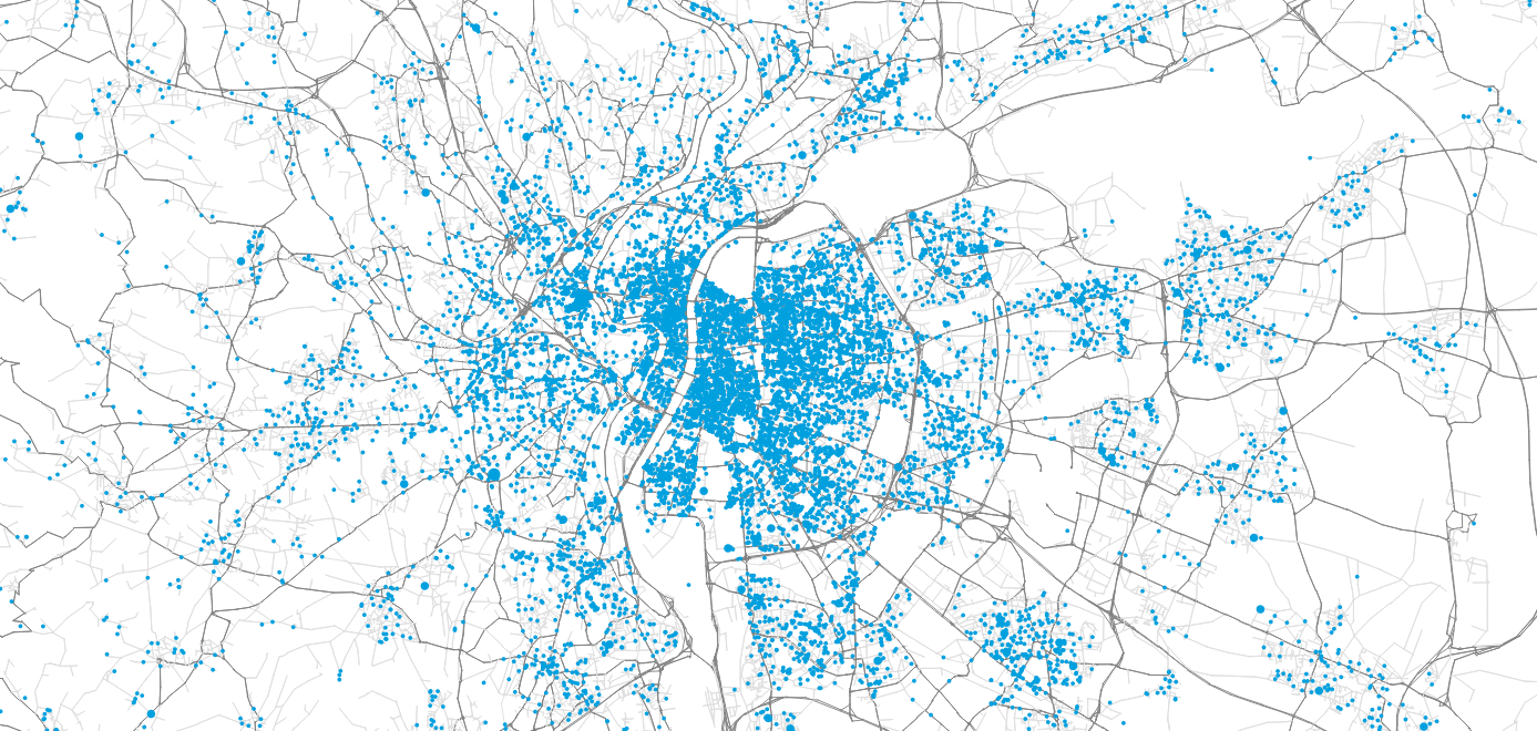
- Example: Sampling trips in Paris
- The sampling approaches allows for downsampling of the simulation (only simulating a certain share of movements)
N = 100

Disaggregated demand
- Example: Sampling trips in Paris
- The sampling approaches allows for downsampling of the simulation (only simulating a certain share of movements)
N = 100
N = 1,000

Disaggregated demand
- Example: Sampling trips in Paris
- The sampling approaches allows for downsampling of the simulation (only simulating a certain share of movements)
N = 100
N = 1,000
N = 100,000

N = 10,000
Disaggregated demand
- Sampling of the departure times
- Option 1: We make a hypothesis (here for the morning peak)
t \sim \mathcal{N}(\mu = 8.5, \sigma = 1)


Disaggregated demand
- Sampling of the departure times
- Option 2: We compare with data, or sample directly from data
EGT: Household travel survey for Île-de-France (not open)
ENTD: National household travel survey

Disaggregated demand
- Sampling of the departure times
- Option 2: We compare with data, or sample directly from data
EGT: Household travel survey for Île-de-France (not open)
ENTD: National household travel survey

Mixture of three Gaussians
Disaggregated demand
- Further steps
- Sampling an age for each trip?
- Sampling a socioprofessional category for each trip?
- Sampling which modes of transport are available for each trip?
- Can be conditioned on the distributions in the origin or destination zones
- Remark: This is a common approach when working with Call Detail Records (CDR).
- Operators track the runtime between your phone and surrounding cell towers
- Having at least three towers allows for approximate triangulation of your position
- Since each phone has an ID, a trajectory can be constructed per user
- BUT: The ID must be anonymized and GDPR forbids attaching user information
- However, the traces can be enriched by statistical data
Disaggregated demand
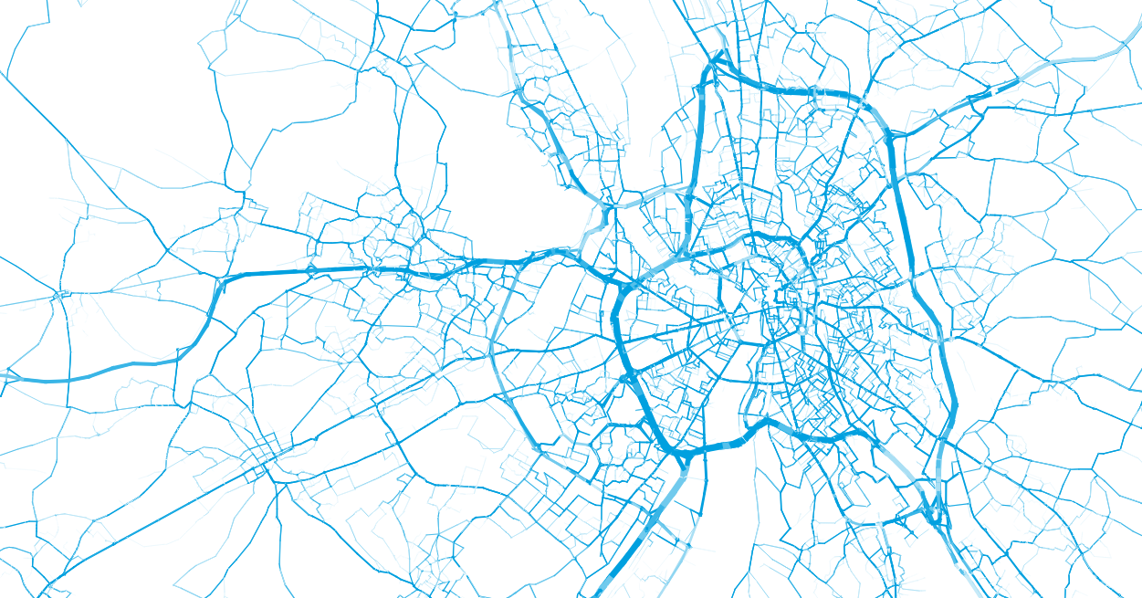
- Given that we have origin and destination coordinates, we can now perform a detailed routing of the trips on the road network, for instance by finding the shortest (in terms of distance) path.
N = 100
N = 1,000
N = 10,000

Disaggregated demand
- Given that we have origin and destination coordinates, we can now perform a detailed routing of the trips on the road network, for instance by finding the shortest (in terms of distance) path.
N = 100
N = 1,000
N = 10,000

Disaggregated demand
- Given that we have origin and destination coordinates, we can now perform a detailed routing of the trips on the road network, for instance by finding the shortest (in terms of distance) path.
N = 100
N = 1,000
N = 10,000

Disaggregated demand
- Given that we have origin and destination coordinates, we can now perform a detailed routing of the trips on the road network, for instance by finding the shortest (in terms of distance) path.
N = 100
N = 1,000
N = 10,000

Disaggregated demand
- Given that we have origin and destination coordinates, we can now perform a detailed routing of the trips on the road network, for instance by finding the shortest (in terms of distance) path.
- Common routing algorithms for the road network:
- Dijsktra (from the 50s)
Classic, easy to understand
- A* (from the 60s)
Speed-up through the use of heuristics
- ALT (A*, Landmarks, and Triangle inequality, 2003)
Intelligently constraining the search space of A* for heavy speed-up
- Contraction Hierarchies (2008)
Heavy preprocessing of the network, but very fast lookup of routes
- Dijsktra (from the 50s)
Disaggregated demand
- Given that we have origin and destination coordinates, we can now perform a detailed routing of the trips on the road network, for instance by finding the shortest (in terms of distance) path.
- Common routing algorithms for the transit network:
- Time-extended Dijkstra
Long time standard approach, very time and memory consuming
- RAPTOR
Standard today, labelling algorithm
- Connection scan (2015)
Intelligent arrangement of transit schedules in memory
- Time-extended Dijkstra
Disaggregated demand
- From the 2000s, change of paradigm:
Disaggregated demand
- From the 2000s, change of paradigm:
Transport demand is generated by the need of people to perform activities
Disaggregated demand
- From the 2000s, change of paradigm:
- This change of perspective lead to activity-based models
- Individual persons are modelled (which individual attributes like age, CSP, ...)
Transport demand is generated by the need of people to perform activities


x 12,000,000
Disaggregated demand
- From the 2000s, change of paradigm:
- This change of perspective lead to activity-based models
- Individual persons are modelled (which individual attributes like age, CSP, ...)
- Each person has a chain of activities during the day (home - work - shopping - home)
- Individual persons are modelled (which individual attributes like age, CSP, ...)
Transport demand is generated by the need of people to perform activities


Disaggregated demand
- From the 2000s, change of paradigm:
- This change of perspective lead to activity-based models
- Individual persons are modelled (which individual attributes like age, CSP, ...)
- Each person has a chain of activities during the day (home - work - shopping - home)
- Each activity has specific coordinates and a time at which it should happen
- Individual persons are modelled (which individual attributes like age, CSP, ...)
Transport demand is generated by the need of people to perform activities
0:00 - 9:00
10:00 - 17:30
17:45 - 21:00
22:00 - 0:00
Disaggregated demand
- From the 2000s, change of paradigm:
- This change of perspective lead to activity-based models
- Individual persons are modelled (which individual attributes like age, CSP, ...)
- Each person has a chain of activities during the day (home - work - shopping - home)
- Each activity has specific coordinates and a time at which it should happen
- Activities are connected by trips that bring people from A to B (with a specific transport mode)
- Individual persons are modelled (which individual attributes like age, CSP, ...)
Transport demand is generated by the need of people to perform activities


0:00 - 9:00
10:00 - 17:30
17:45 - 21:00
22:00 - 0:00
Disaggregated demand
- The approach results in data sets that are useful for many different domains
-
Synthetic population: Households, persons and their sociodemographic attributes
-
Synthetic demand: Activity chains for each person
-
Synthetic population: Households, persons and their sociodemographic attributes
- Models can be set up for
- Energy consumption of the population
- Evacuation of natural disasters
- Spread of diseases and epidemics (heavily used during Covid-19!)
- Of course, transport planning and simulation
- Energy consumption of the population
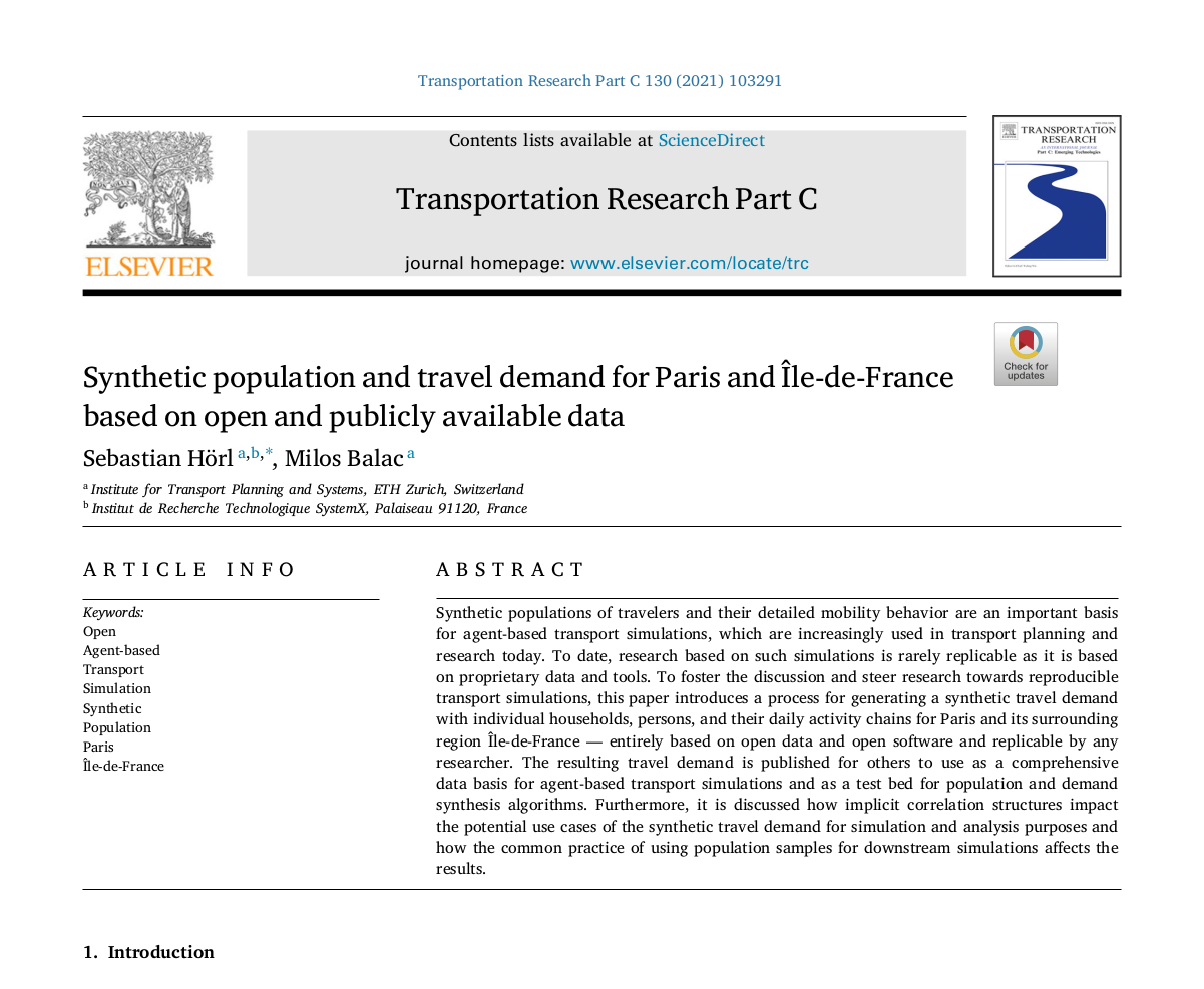
2.2 Synthetic travel demand for France
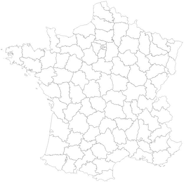
Synthetic travel demand for France

Population census (RP)
> Truncate-Replicate-Sample (TRS)
Synthetic travel demand for France
Population census (RP)
Income data (FiLoSoFi)

> Imputation by quantile
Synthetic travel demand for France
Population census (RP)
Income data (FiLoSoFi)
Commuting data (RP-MOB)

> Direct sampling from OD matrix
Synthetic travel demand for France
Population census (RP)
Income data (FiLoSoFi)
Commuting data (RP-MOB)

Household travel survey (EDGT)

0:00 - 8:00
08:30 - 17:00
17:30 - 0:00
0:00 - 9:00
10:00 - 17:30
17:45 - 21:00
22:00 - 0:00
> Assignment of activity chains through statistical matching
Synthetic travel demand for France
Population census (RP)
Income data (FiLoSoFi)
Commuting data (RP-MOB)
Household travel survey (EDGT)
Enterprise census (SIRENE)


Address database (BD-TOPO)
> Specifically designed approach to find secondary locations
Hörl, S., Axhausen, K.W., 2021. Relaxation–discretization algorithm for spatially constrained secondary location assignment. Transportmetrica A: Transport Science 1–20. https://doi.org/10.1080/23249935.2021.1982068
Synthetic travel demand for France
Population census (RP)
Income data (FiLoSoFi)
Commuting data (RP-MOB)
Household travel survey (EDGT)
Enterprise census (SIRENE)
Address database (BD-TOPO)
Person ID
Age
Gender
Home (X,Y)
1
43
male
(65345, ...)
2
24
female
(65345, ...)
3
9
female
(65345, ...)
Synthetic travel demand for France
Population census (RP)
Income data (FiLoSoFi)
Commuting data (RP-MOB)
Household travel survey (EDGT)
Enterprise census (SIRENE)
Address database (BD-TOPO)
Person ID
Activity
Start
End
Loc.
523
home
08:00
(x,y)
523
work
08:55
18:12
(x,y)
523
shop
19:10
19:25
(x,y)
523
home
19:40
(x,y)
Synthetic travel demand for France
Population census (RP)
Income data (FiLoSoFi)
Commuting data (RP-MOB)
Household travel survey (EDGT)
Enterprise census (SIRENE)
OpenStreetMap
GTFS (SYTRAL / SNCF)
Address database (BD-TOPO)
Synthetic travel demand for France
Population census (RP)
Income data (FiLoSoFi)
Commuting data (RP-MOB)
National HTS (ENTD)
Enterprise census (SIRENE)
OpenStreetMap
GTFS (SYTRAL / SNCF)
Address database (BD-TOPO)
EDGT
Synthetic travel demand for France
Population census (RP)
Income data (FiLoSoFi)
Commuting data (RP-MOB)
National HTS (ENTD)
Enterprise census (SIRENE)
OpenStreetMap
GTFS (SYTRAL / SNCF)
Address database (BD-TOPO)
EDGT
Open
Data

Open
Software
+
=
Reproducible research
Integrated testing
Synthetic travel demand for France
Population census (RP)
Income data (FiLoSoFi)
Commuting data (RP-MOB)
National HTS (ENTD)
Enterprise census (SIRENE)
OpenStreetMap
GTFS (SYTRAL / SNCF)
Address database (BD-TOPO)
EDGT
Open
Data
Open
Software
+
=
Reproducible research
Integrated testing
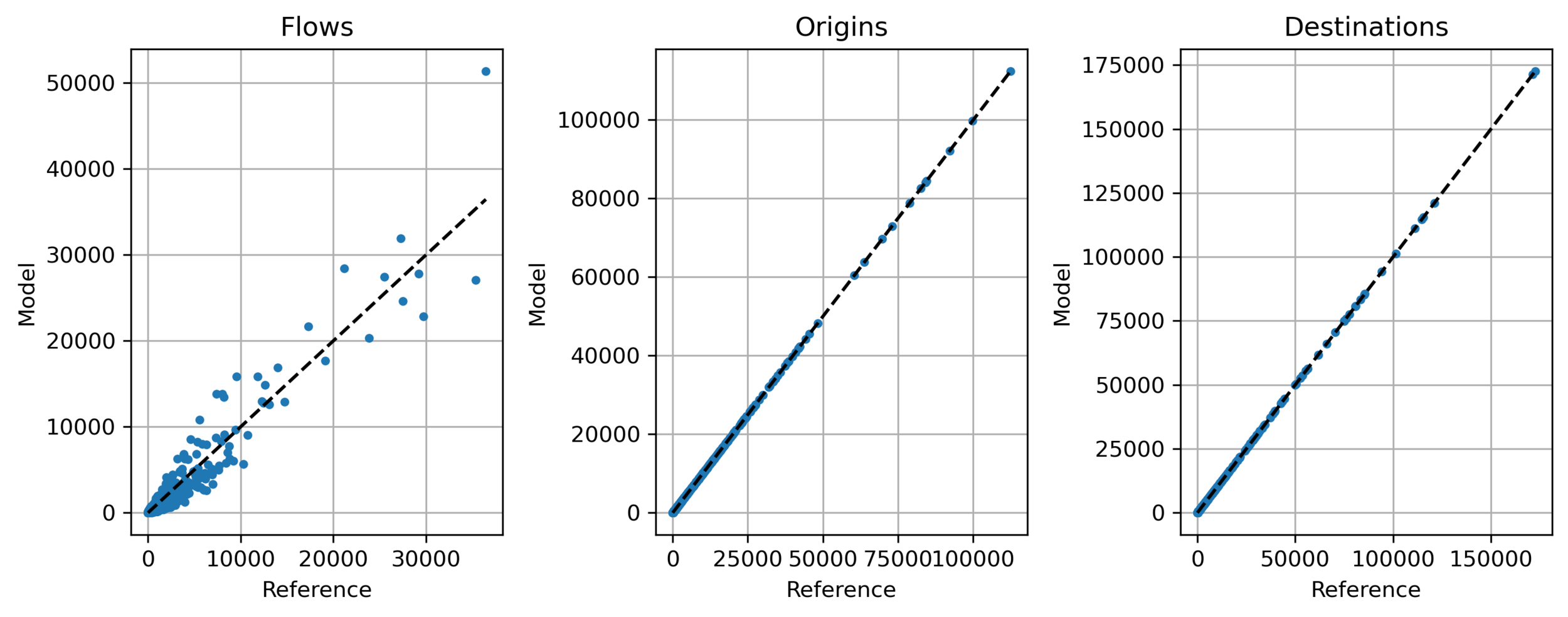
Synthetic travel demand for France

- Comparison of population attributes
Synthetic travel demand for France

- Activity chains
Synthetic travel demand for France


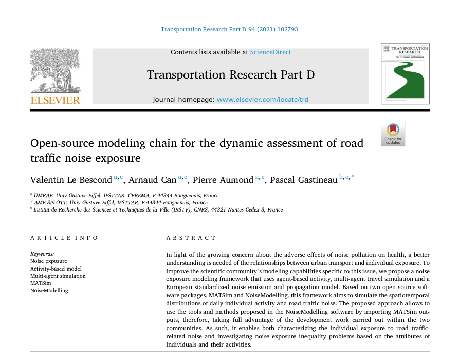
Synthetic travel demand for France

Nantes
- Noise modeling
Synthetic travel demand for France
Lille
- Park & ride applications
- Road pricing

Synthetic travel demand for France

Toulouse
- Placement and use of shared offices
Synthetic travel demand for France
Rennes
- Micromobility simulation

Synthetic travel demand for France

Paris / Île-de-France
- Scenario development for sustainable urban transformation
- New mobility services
Mahdi Zargayouna (GRETTIA / Univ. Gustave Eiffel)
Nicolas Coulombel (LVMT / ENPC)
Synthetic travel demand for France


Paris / Île-de-France
- Cycling simulation
Synthetic travel demand for France
Paris / Île-de-France
- Simulation of dynamic mobility services
- Fleet control through reinforcement learning
Synthetic travel demand for France

Lyon (IRT SystemX)
- Low-emission first/last mile logistics
Synthetic travel demand for France

Synthetic travel demand for France
Balac, M., Hörl, S. (2021) Synthetic population for the state of California based on open-data: examples of San Francisco Bay area and San Diego County, presented at 100th Annual Meeting of the Transportation Research Board, Washington, D.C.
Sallard, A., Balac, M., Hörl, S. (2021) Synthetic travel demand for the Greater São Paulo Metropolitan Region, based on open data, Under Review
Sao Paulo, San Francisco Bay area, Los Angeles five-county area, Switzerland, Montreal, Quebec City, Jakarta, Casablanca, ...
Synthetic travel demand for France
- Latest addition: Cairo
- Germany work-in-progress
Synthetic travel demand for France
- Reproducibility
- Low in transport modelling / simulation, especially with agent-based models
- Can increase acceptance, uptake and more widespread use of these models
- Increasingly available open data sources make reproducibility possible, but processes aren't standardized or not easily accessible as open source
- Our goal: Have pipeline from raw data to a calibrated large-scale agent-based transport simulation that is nearly 100% replicable with reproducible results.

Synthetic travel demand for France
- Continuously updated
- Example: Integrating buildings
- Open data: BAN (Base d'addresses nationale)
- Open data: BD-TOPO building census
- Benchmarking methodology
- Bayesian networks, HMMs, deep learning, ...
Synthetic travel demand for France
- 5% Sample of the data is available on Mendeley
3.1 Agent-based transport simulation
Agent-based transport simulation
- Previously, we have seen how one can generate disaggregated synthetic travel demand
- Such demand data sets are used in agent-based simulation
Agent-based transport simulation
- One option: microscopic simulation
- Each agent is simulated in detail
- Cars have a location
- Velocity and acceleration
- They move according to what they perceive around them
Agent-based transport simulation
- One option: microscopic simulation
- Each agent is simulated in detail
- Cars have a location
- Velocity and acceleration
- They move according to what they perceive around them
- A commonly used model is the Intelligent Driver Model

Agent-based transport simulation
- One option: microscopic simulation
- Each agent is simulated in detail
- Cars have a location
- Velocity and acceleration
- They move according to what they perceive around them
- A commonly used model is the Intelligent Driver Model
is your current speed, and is the speed limit
v_\alpha
v_0
Agent-based transport simulation
- One option: microscopic simulation
- Each agent is simulated in detail
- Cars have a location
- Velocity and acceleration
- They move according to what they perceive around them
- A commonly used model is the Intelligent Driver Model
is your current distance to the leading car , and is the desired distance
s_\alpha
s^*
Agent-based transport simulation
- This video shows the driver behavior that is modeled by the IDM
Agent-based transport simulation
- Microscopic models
- Represent traffic in high detail
- Are highly realistic
- Can be calibrated directly on driver behavior (drone videos, ...)
- But
- Are computational heavy!
- Need to be simulated on a sub-second basis
- With many cars (12M agents in Île-de-France, this becomes infeasible!)
Agent-based transport simulation
- Other option: Mesoscopic models
- Agents interact with a network that consists of vertices and edges (nodes and links)
- Agents move through one link and then wait at the end to be transferred to the next one
- If there is no space on the next link, agents may be blocked temporarily, thus creating a traffic jam
3.2 MATSim
MATSim
- Flexible, extensible and well-tested open-source transport simulation framework
- Used by many research groups and companies all over the world
- Extensions for parking behaviour, signal control, location choice, freight, ...

http://www.matsim.org
matsim-org/matsim-libs


MATSim
- Flexible, extensible and well-tested open-source transport simulation framework
- Used by many research groups and companies all over the world
- Extensions for parking behaviour, signal control, location choice, freight, ...
http://www.matsim.org
matsim-org/matsim-libs
MATSim
- Two major components
-
Mobility simulation: mesoscopic simulation of all movements in the transport system
- Decision-making: agents tracking how well their routing and mode decisions worked, then making new decisions
Mobility simulation
Decision-making
Analysis
Scenario
MATSim
- Flexible, extensible and well-tested open-source transport simulation framework
- Used by many research groups and companies all over the world
- Extensions for parking behaviour, signal control, location choice, freight, ...
Mobility simulation
Decision-making
Analysis
Scenario
MATSim
- Link-based mobility simulation
- Each link consists of a queue and a buffer
- Vehicles enter the queue and wait until they are allowed to pass through the link (flow capacity) into the buffer
- Vehicles wait inside the buffer until there is space (storage capacity) on the next link of their route
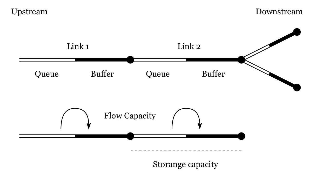
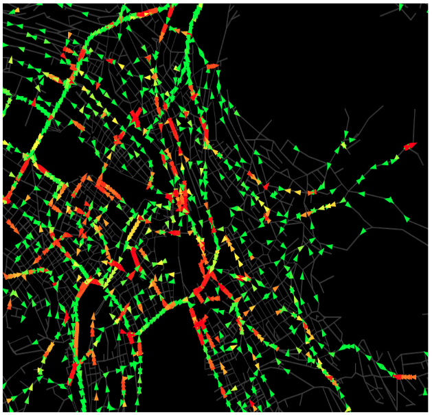
MATSim
-
Decision-making is based on two concepts
-
Scoring: Agents track how their daily plan works (delays? congestion?)
- Agents gain positive score when performing activities at the time they are planned, and lose score when they spend time in transport
- Similar to the utility concept of mode choice models
- Replanning: Agents keep a memory of past observed plans and select among them or introduce small changes (change transport mode, depart earlier, ...)
MATSim
MATSim
- A basic MATSim simulation needs two major inputs: plans and a network
- A plans file in XML format that describes the daily schedule of each person
MATSim
- A basic MATSim simulation needs two major inputs: plans and a network
- A plans file in XML format that describes the daily schedule of each person

MATSim
- A basic MATSim simulation needs two major inputs: plans and a network
- A plans file in XML format that describes the daily schedule of each person
- A plans file can be generated by directly writing out a trip table as XML

MATSim
- A basic MATSim simulation needs two major inputs: plans and a network
- A network file describes the road network as edges and nodes
MATSim
- A basic MATSim simulation needs two major inputs: plans and a network
- A network file describes the road network as edges and nodes

MATSim
- A basic MATSim simulation needs two major inputs: plans and a network
- A network file describes the road network as edges and nodes

MATSim
- MATSim can either be configured using an XML-based configuration file or a directly inside the code. A common run script looks as follows:

MATSim
- In a full MATSim simulation, agents would choose between different modes, routes, etc.
- But one can also simply run one iteration to track the movements of the vehicles
MATSim
- The main output of MATSim is the events file that contains everything that happens during the simulation
- By aggregating this file, we can obtain any relevant information
MATSim
- The main output of MATSim is the events file that contains everything that happens during the simulation
- By aggregating this file, we can obtain any relevant information

MATSim
- The main output of MATSim is the events file that contains everything that happens during the simulation
- By aggregating this file, we can obtain any relevant information
- But there are pre-aggregated data sets, such as the trip table

3.3 On-demand service simulation
On-demand service simulation
- Coming soon
- Initially from the field of operations research
- Traveling salesman problem
- Vehicle routing problem
- Dial-a-ride problem
- Hard to solve! Limited ability for large instances!
- Heuristic approaches needed (1) in reality and (2) especially in simulation: Want to apply approaches that are realistic enough to give some insight, but quick enough to perform simulations (cf. human taxi drivers)
- Simplest approach: Best-response assignment
- Vehicle perspective, passenger perspective, combined
- Adaptive switching
- Bipartite matching approach, many others exist (see recent advances in reinforcement learning)
- Relocation: Strongly linked problem, where to send empty vehicles?
- Show comparison results from Zurich study
Questions?
sebastian.horl@irt-systemx.fr
Large-scale models and simulation methods
By Sebastian Hörl
Large-scale models and simulation methods
Université Gustave Eiffel, Spring 2024


