Sebastian Ordoñez-Soto
Universidad Nacional de Colombia
Internship tutor: Sergey Barsuk
June 27th, 2024
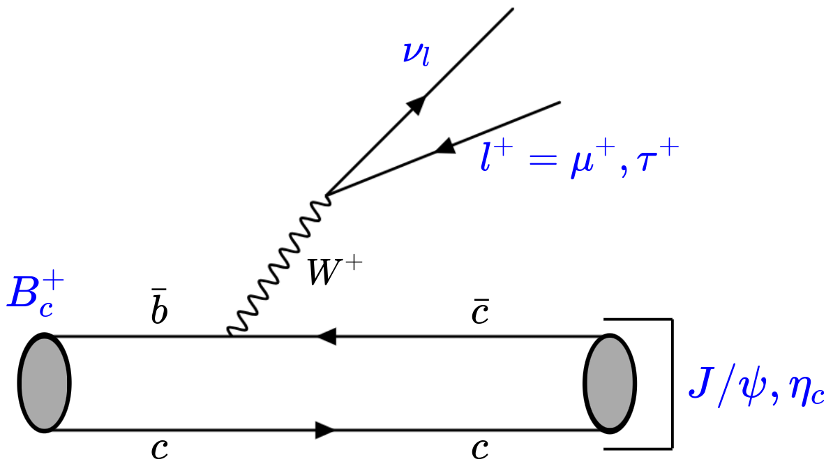
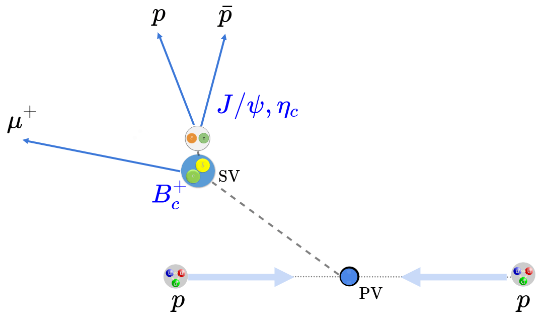
Study and search of the \(B_{c}^{+}\rightarrow (\eta_{c}\rightarrow p\bar{p})\mu^{+}\nu_{\mu}\) decay
IJCLab LHCb group meeting


Outline
- Introduction
- The \(B_{c}\) meson
- \(B_{c}\) semileptonic decays
- Dataset
- Data sample
- MC samples
- Selection
- Pre-selection
- Charmonia optimization
- Analysis
- Fit models
- Signal extraction
- Final fit
- Summary
S. Ordonez Soto
June 27th, 2024
S. Ordonez Soto
June 27th, 2024
Introduction
\(m_{B_{c}} = (6274.47 \pm 0.32)\) MeV
\(\tau_{B_{c}} = (0.507 \pm 0.009) \) ps
-
Lowest-mass bound state of two heavy quarks of different flavors.
-
Discovered by the CDF collaboration in 1998.
-
Has no strong or electromagnetic decay channels.
-
Its weak decay yields a large branching fraction to final states containing a \(J/ \psi\)
-
-
Full decay width: \(\Gamma = \Gamma_{b} + \Gamma_{c} + \Gamma_{bc}\)
-
\(\Gamma_{b}: \bar{b}\rightarrow \bar{c}W^{+}\), with \(c\) as spectator (~ 20%)
-
\(\Gamma_{c}: c\rightarrow sW^{+}\), with \(\bar{b}\) as spectator (~ 70%)
-
\(\Gamma_{bc}: c\bar{b} \rightarrow W^{+}\), weak annihilation (~ 10%)
-
Introducing the \(B_{c}^{+}\) meson
\longrightarrow
\longrightarrow
\longrightarrow
(c\bar{c}) l \nu_{l}
,(c\bar{c}) \pi, ...
B_{s} \pi, B_{s}l\nu_{l}, ...
D^{*}K^{+}, ...

S. Ordonez Soto
June 27th, 2024
Introduction
The decay channel
-
\(B_{c}^{+}\rightarrow \eta_{c}\mu^{+}\nu_{\mu}\) is one of the possible \(B_{c}^{+}\) semileptonic (SL) decay channels.
- Full width determination
- Lepton Flavor Universality test \(\rightarrow R(\eta_{c})\)
-
\(B_{c}^{+}\rightarrow J/\psi\mu^{+}\nu_{\mu}\) was already measured by LHCb \(\rightarrow R(J/\psi)\).
S. Ordonez Soto
June 27th, 2024
Introduction
Analysis strategy
-
The \(B_{c}^{+}\rightarrow \eta_{c}\mu^{+}\nu_{\mu}\) decay will be analyzed together with the \(B_{c}^{+}\rightarrow J/\psi\mu^{+}\nu_{\mu}\), which is used as normalization channel.
-
The ratio \(\frac{\mathcal{B}(B_{c}^{+}\rightarrow \eta_{c}\mu^{+}\nu_{\mu})}{\mathcal{B}(B_{c}^{+}\rightarrow J/\psi\mu^{+}\nu_{\mu})}\) can be calculated as:
Calculated from MC
Yield extraction from final fit
\boxed{\frac{\mathcal{B}(B_{c}^{+}\rightarrow \eta_{c}\mu^{+}\nu_{\mu})}{\mathcal{B}(B_{c}^{+}\rightarrow J/\psi\mu^{+}\nu_{\mu})} =
\frac{N_{B_{c}^{+}\rightarrow \eta_{c}\mu^{+}\nu_{\mu}}}{N_{B_{c}^{+}\rightarrow J/\psi\mu^{+}\nu_{\mu}}} \times
\frac{\mathcal{B}(J/\psi \rightarrow p\bar{p})}{\mathcal{B}(\eta_{c}\rightarrow p\bar{p})} \times
\frac{\epsilon_{tot}(B_{c}^{+}\rightarrow \eta_{c}\mu^{+}\nu_{\mu})}{\epsilon_{tot}(B_{c}^{+}\rightarrow J/\psi\mu^{+}\nu_{\mu})}}
-
The \(R_{\eta_{c}}\) could be calculated as:
\boxed{R_{\eta_{c}}=\frac{\mathcal{B}(B_{c}^{+}\rightarrow \eta_{c}\mu^{+}\nu_{\mu})}{\mathcal{B}(B_{c}^{+}\rightarrow J/\psi\mu^{+}\nu_{\mu})} \times
\frac{\mathcal{B}(B_{c}^{+}\rightarrow J/\psi\tau^{+}\nu_{\tau})}{\mathcal{B}(B_{c}^{+}\rightarrow \eta_{c}\tau^{+}\nu_{\tau})} \times
\frac{1}{R_{J/\psi}}}
S. Ordonez Soto
June 27th, 2024
Dataset
Data sample
LHCb run 2 data from proton-proton collisions, at \(\sqrt{s}=13 \text{TeV}\) and \(4 \text{fb}^{-1}\), collected from 2015 to 2017.
-
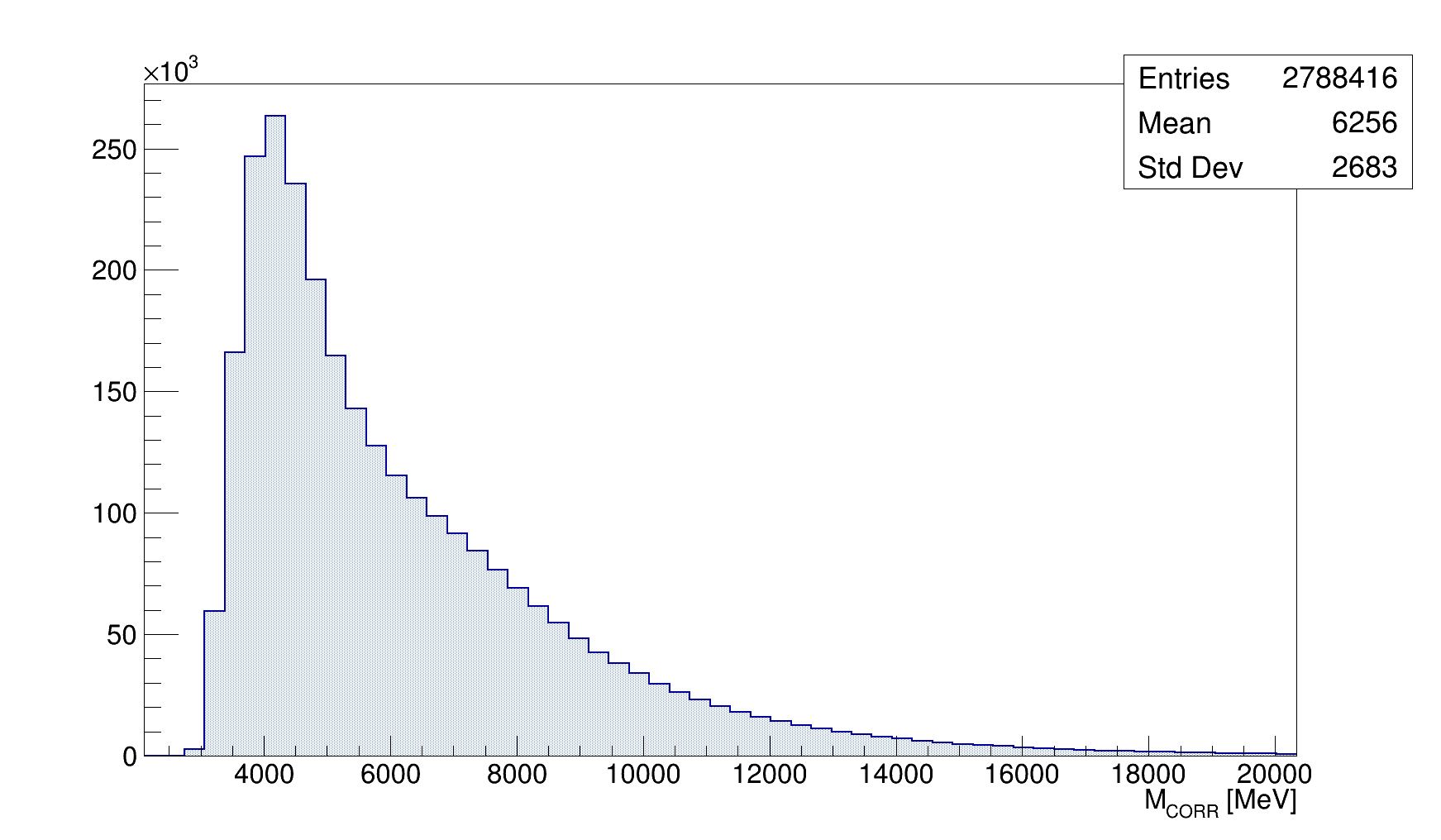
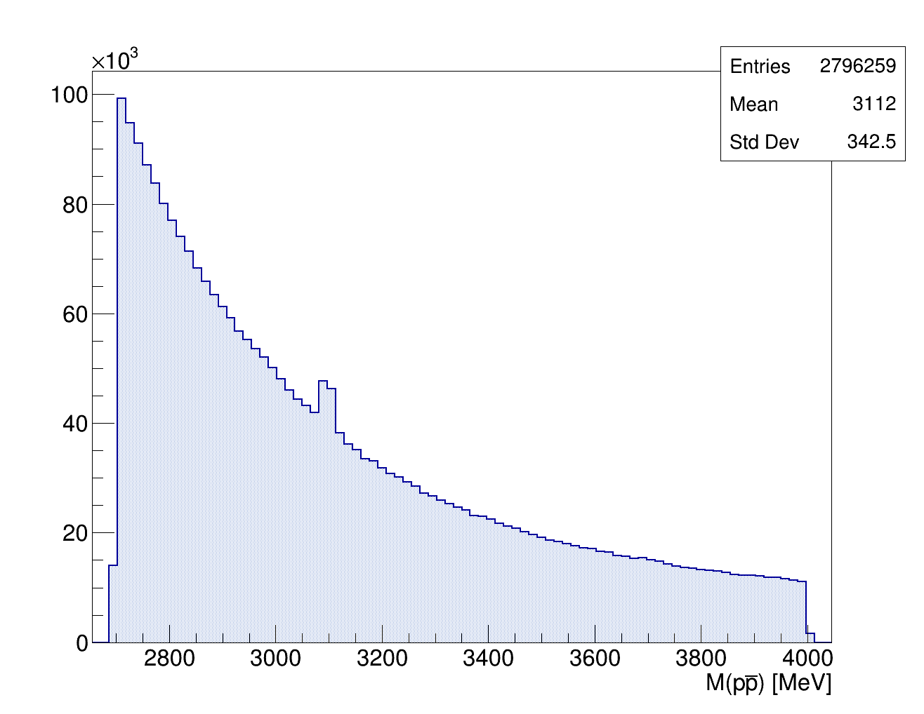
There are two main variables for the analysis:
-
The \(p\bar{p}\) invariant mass \(M(p\bar{p})\)
-
The \(p\bar{p}\mu\) corrected mass, defined as: \(M_{CORR} = \sqrt{M^{2}(p\bar{p}\mu) + p^{2}_{\bot}} + p_{\bot}\)
-
S. Ordonez Soto
June 27th, 2024
Simulation samples
There are Monte Carlo samples available for both signal and different backgrounds
Dataset
B_{c}^{+}\rightarrow (h_{c}\rightarrow \eta_{c}\gamma)\mu^{+}\nu_{\mu}
B_{c}^{+}\rightarrow \eta_{c}(\tau^{+}\rightarrow\mu^{+}\nu_{\mu}\bar{\nu}_{\tau})\nu_{\tau}
B_{c}^{+}\rightarrow (\psi(2S)\rightarrow J/\psi\pi^{+}\pi^{-})\mu^{+}\nu_{\mu}
B_{c}^{+}\rightarrow J/\psi(\tau^{+}\rightarrow\mu^{+}\nu_{\mu}\bar{\nu}_{\tau})\nu_{\tau}
B_{c}^{+}\rightarrow (\chi_{c0}\rightarrow J/\psi\gamma)\mu^{+}\nu_{\mu}
\eta_{c} \hspace{0.1cm} \text{peaking bkg.}
J/\psi \hspace{0.1cm }\text{peaking bkg.}
B_{c}^{+}\rightarrow (\chi_{c1}\rightarrow J/\psi\gamma)\mu^{+}\nu_{\mu}
B_{c}^{+}\rightarrow (\chi_{c2}\rightarrow J/\psi\gamma)\mu^{+}\nu_{\mu}
- Signal: \(B_{c}^{+}\rightarrow (\eta_{c}\rightarrow p\bar{p})\mu^{+}\nu_{\mu}\) and \(B_{c}^{+}\rightarrow (J/\psi\rightarrow p\bar{p})\mu^{+}\nu_{\mu}\)
-
Background:
-
Inclusive bkg: \(b\rightarrow \eta_{c}X\) and \(b\rightarrow J/\psi X\) decays
-
Peaking bkg:
-
S. Ordonez Soto
June 27th, 2024
Selection
Pre-selection
Charmonia optimization
A set of selection requirements is initially applied, including: vertex quality and PID requirements
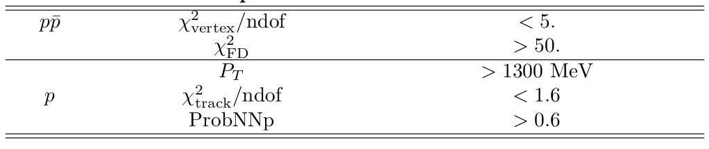
Additional cuts are added to optimize charmonia:
S. Ordonez Soto
June 27th, 2024
Analysis
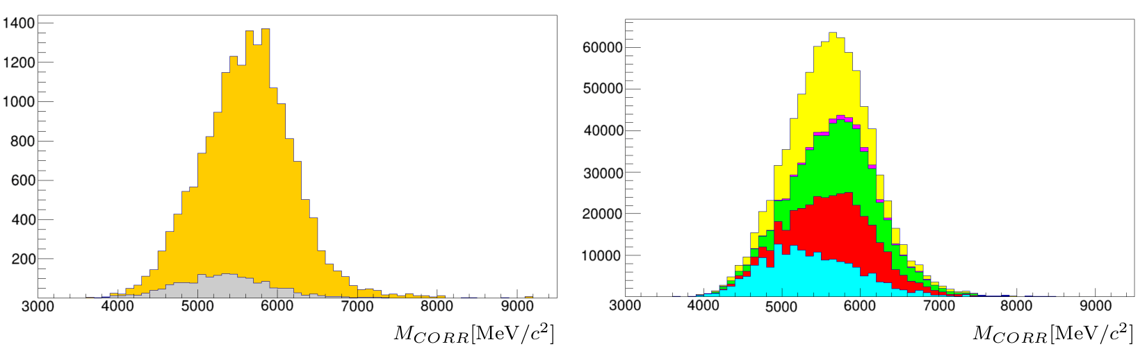
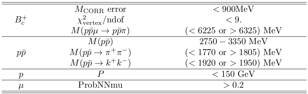
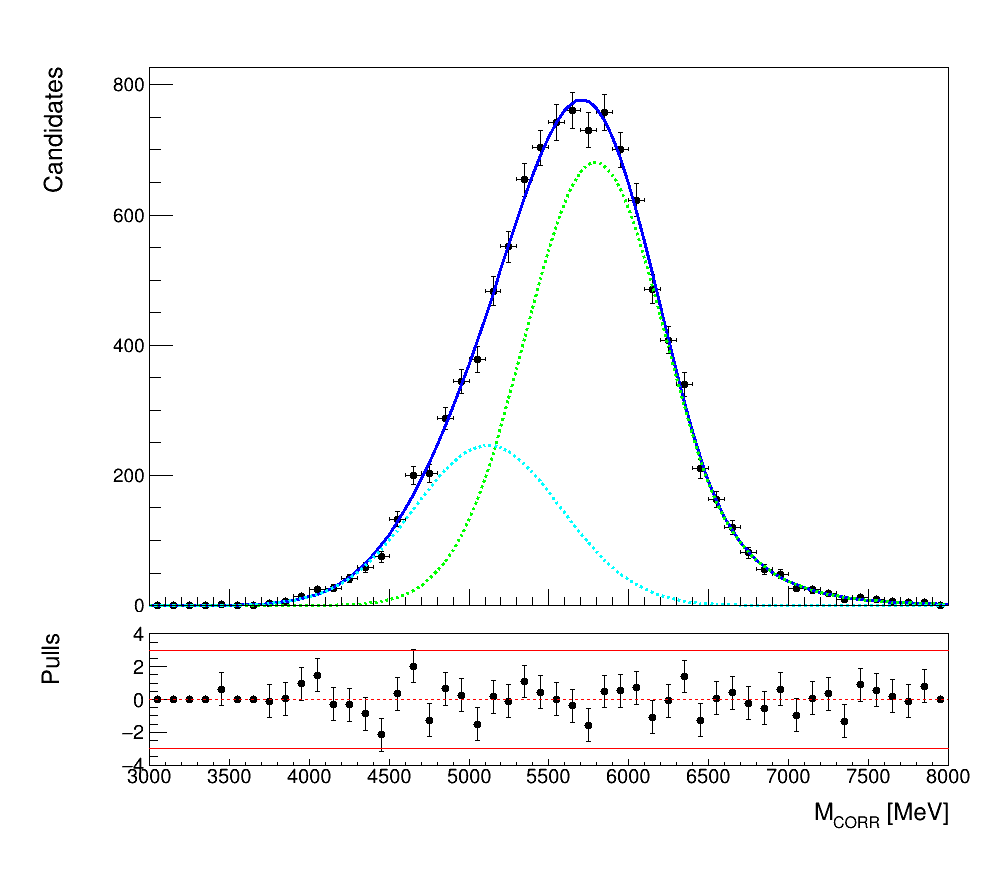
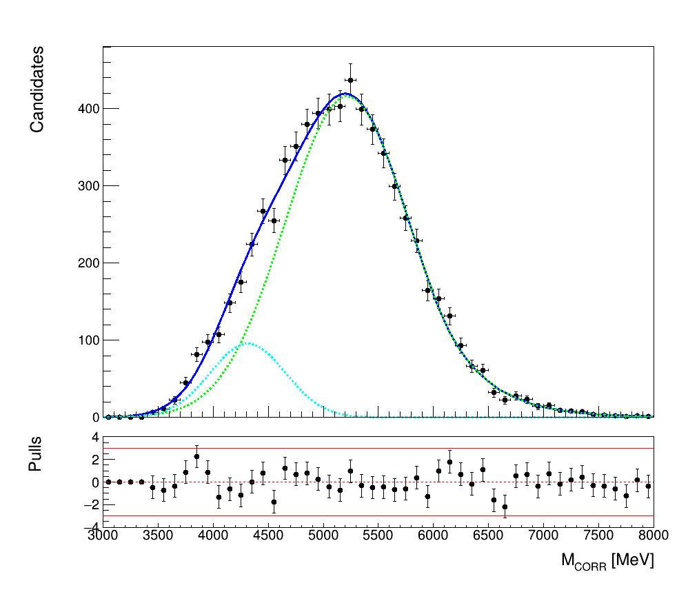
Fit models to \(M_{CORR}\) distributions
Using the MC samples the shapes of the \(M_{CORR}\) distributions for signal and background decay channels are extracted.
- Signal:
\(B_{c}^{+}\rightarrow\eta_{c}\mu^{+}\nu_{\mu}\)
\(B_{c}^{+}\rightarrow J/\psi\mu^{+}\nu_{\mu}\)
F_{excl,sig} (M_{CORR}) = f \cdot CB(M_{CORR};\mu_{1},R,\alpha,n) + (1-f) \cdot G(M_{CORR};\mu_{1}+d,\sigma_{1})
S. Ordonez Soto
June 27th, 2024
Analysis
Fit models to \(M_{CORR}\) distributions
- \(\eta_{c}\) peaking background:
\(B_{c}\rightarrow(\chi_{0}\rightarrow J/\psi\gamma)\mu\nu_{\mu}\)
\(B_{c}\rightarrow(\chi_{1}\rightarrow J/\psi\gamma)\mu\nu_{\mu}\)
\(B_{c}\rightarrow(\chi_{2}\rightarrow J/\psi\gamma)\mu\nu_{\mu}\)
\(B_{c}\rightarrow \eta_{c}(\tau\rightarrow\mu\nu_{\mu}\bar{\nu_{\tau}})\nu_{\tau}\)
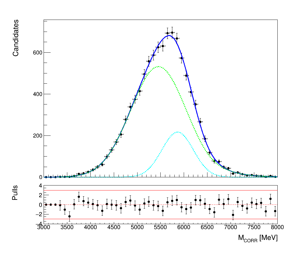
\(B_{c}\rightarrow(h_{c}\rightarrow\eta_{c}\gamma)\mu\nu_{\mu}\)
- \(J/\psi\) peaking background:
\(B_{c}\rightarrow J/\psi(\tau\rightarrow\mu\nu_{\mu}\bar{\nu_{\tau}})\nu_{\tau}\)
\(B_{c}\rightarrow(\psi(2S)\rightarrow J/\psi \pi\pi)\mu\nu_{\mu}\)
S. Ordonez Soto
June 27th, 2024
Analysis
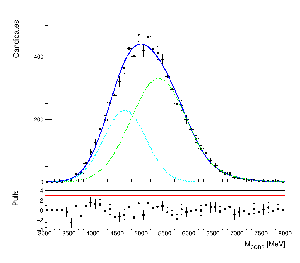
Fit models to \(M_{CORR}\) distributions
F_{incl}(M_{CORR}) = \left(1-\left(\frac{m_{0}}{M_{CORR}}\right)\right)^{p} [f\cdot G(M_{CORR};\mu,\sigma)+(1-f)e^{\alpha\cdot M_{CORR}}]
- Inclusive background
\(b\rightarrow J/\psi X\)
\(b\rightarrow \eta_{c} X\)
S. Ordonez Soto
June 27th, 2024
Analysis
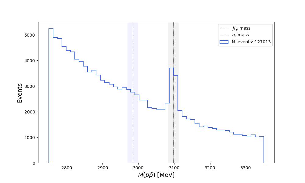
Signal extraction
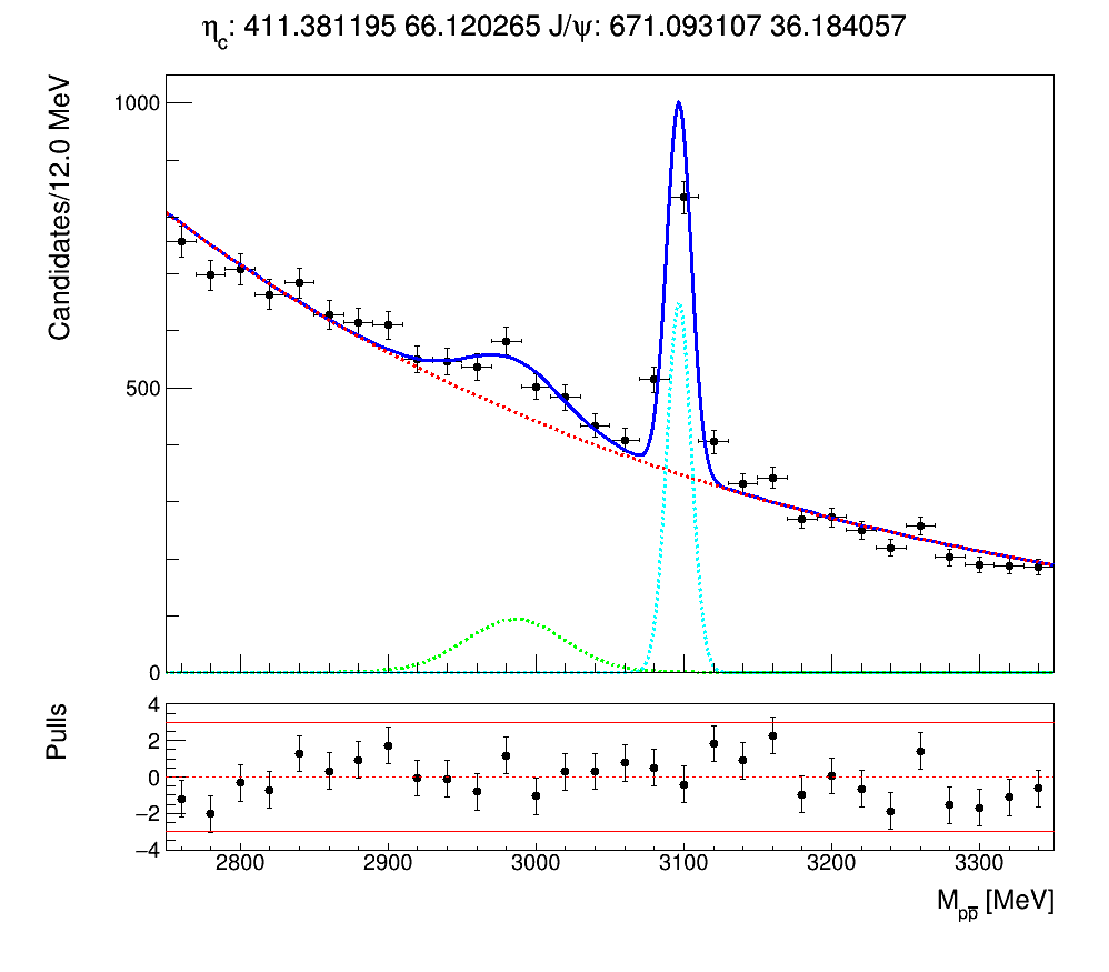
\(\eta_{c}\) and \(J/\psi\) yields are extracted from fits to the \(M(p\bar{p})\) distribution in bins of \(M_{CORR}\)
Data from this bin is extracted, and the charmonia fit model is used
S. Ordonez Soto
June 27th, 2024
Analysis
Signal extraction
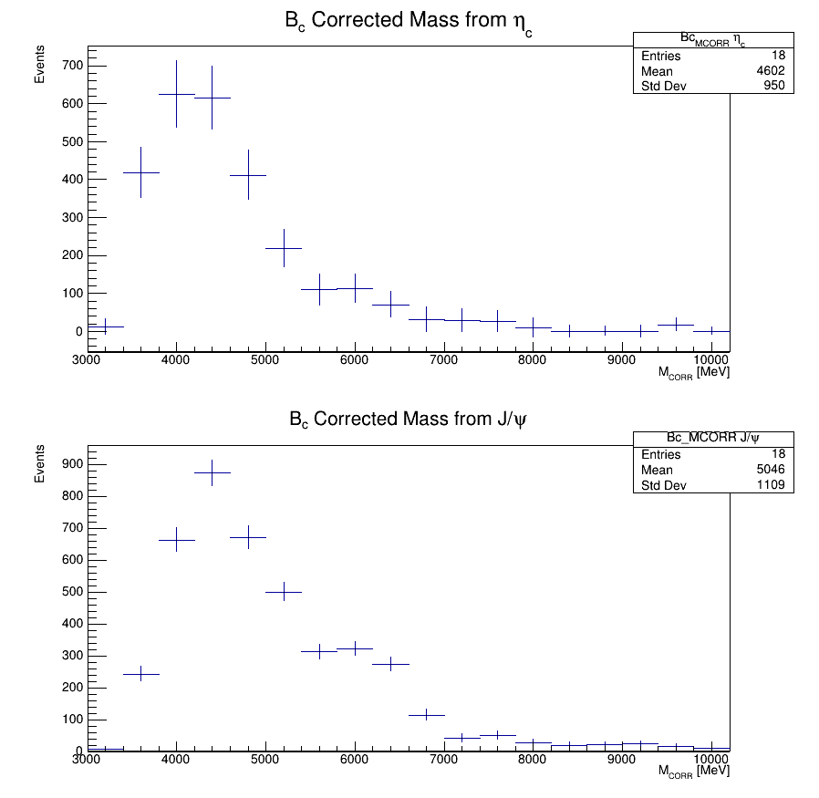
The yields from fits to the \(M(p\bar{p})\) in bins of \(M_{CORR}\) allow us to obtain the \(M_{CORR}\) distribution for true \(\eta_{c}\) and \(J/\psi\)

These true \(\eta_{c}\) and \(J/\psi\) don't necessarily come from \(B_{c}^{+}\rightarrow \eta_{c}\mu^{+}\nu_{\mu}\)
S. Ordonez Soto
June 27th, 2024
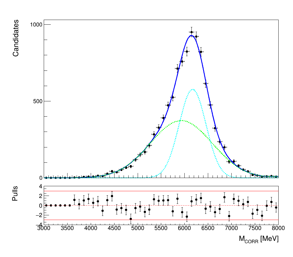
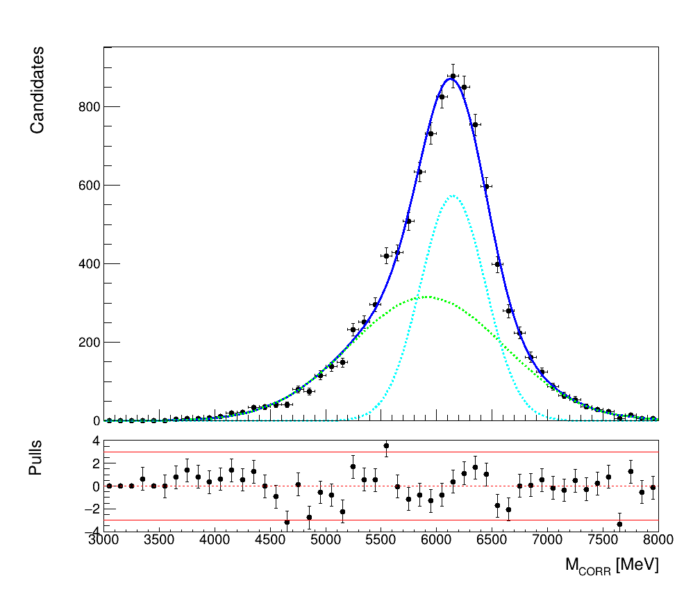
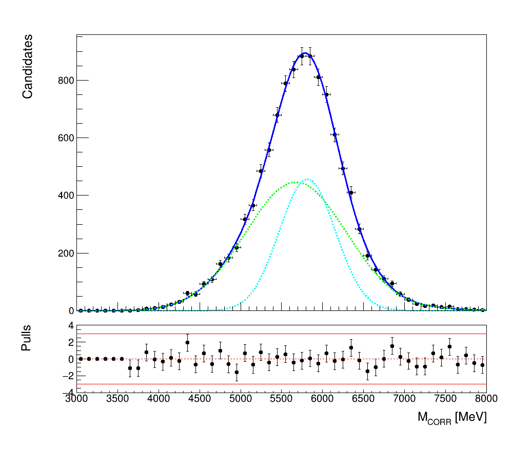
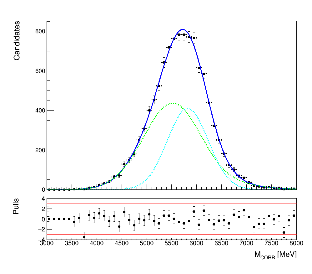
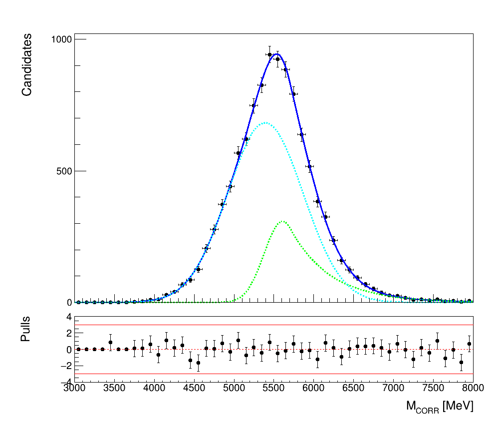
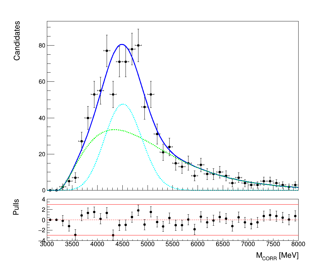
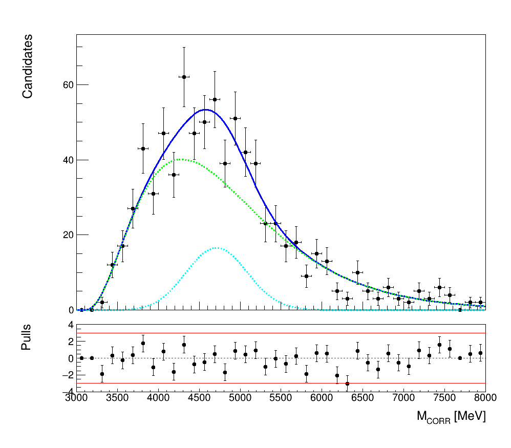
Final fit
Analysis
We use the different shapes to fit these \(M_{CORR}\) distributions and extract the two yields: \(N_{B_{c}^{+}\rightarrow \eta_{c}\mu^{+}\nu_{\mu}}\) and \(N_{B_{c}^{+}\rightarrow J/\psi\mu^{+}\nu_{\mu}}\)
This is work in progress!


\longrightarrow
\boxed{\frac{N_{B_{c}^{+}\rightarrow \eta_{c}\mu^{+}\nu_{\mu}}}{N_{B_{c}^{+}\rightarrow J/\psi\mu^{+}\nu_{\mu}}} = \boxed{?}}
S. Ordonez Soto
June 27th, 2024
Summary
- Review of the different steps of the analysis has be done and implemented.
- A preliminary selection was used which is subject to changes and optimization.
- The shapes of the different signal and background contributions were determined.
- The signal extraction procedure was successfully implemented.
-
Next steps:
- The \(B_{c}^{+}\) optimization is the main next step to complete this preliminary study.
- For next steps would be great to include 2018 data.
S. Ordonez Soto
June 27th, 2024
Thank you for your attention.
Back up
S. Ordonez Soto
June 27th, 2024
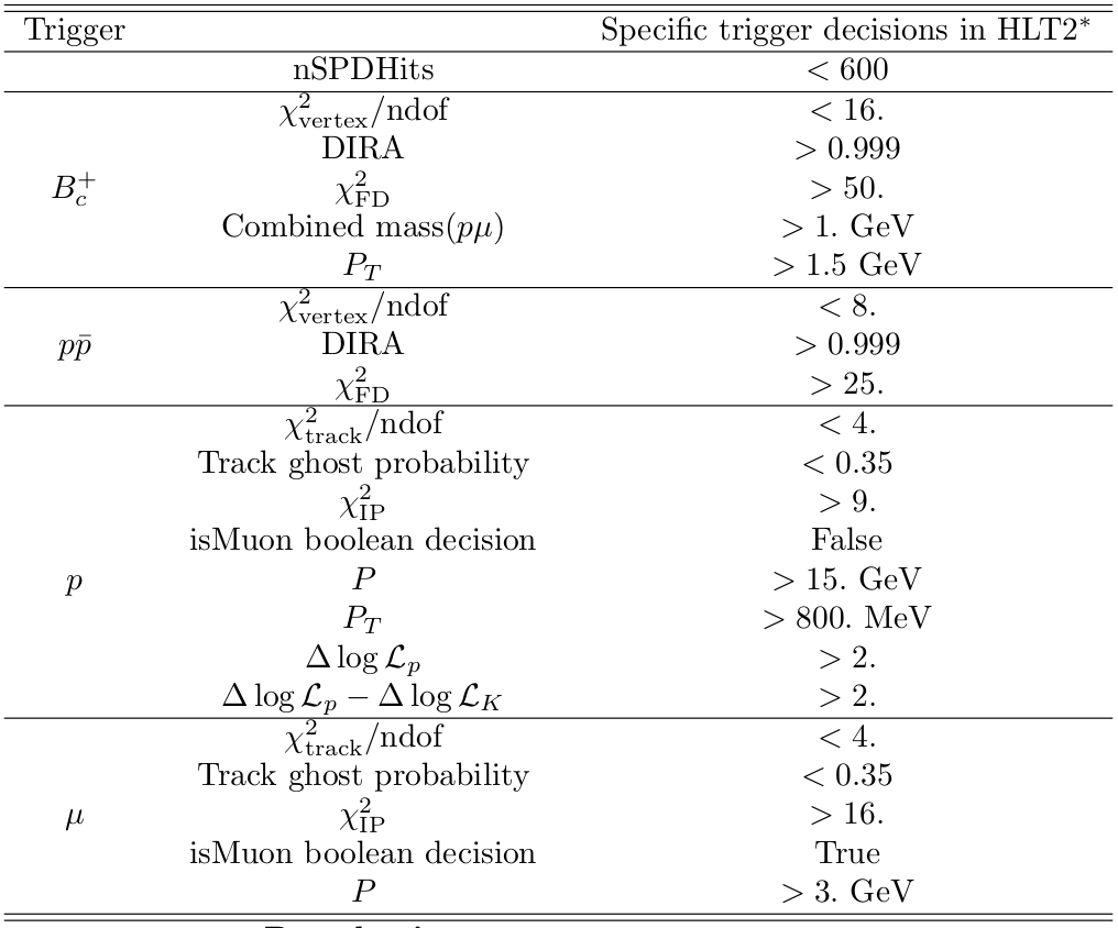
Selection
Stripping selection
S. Ordonez Soto
June 27th, 2024
Analysis
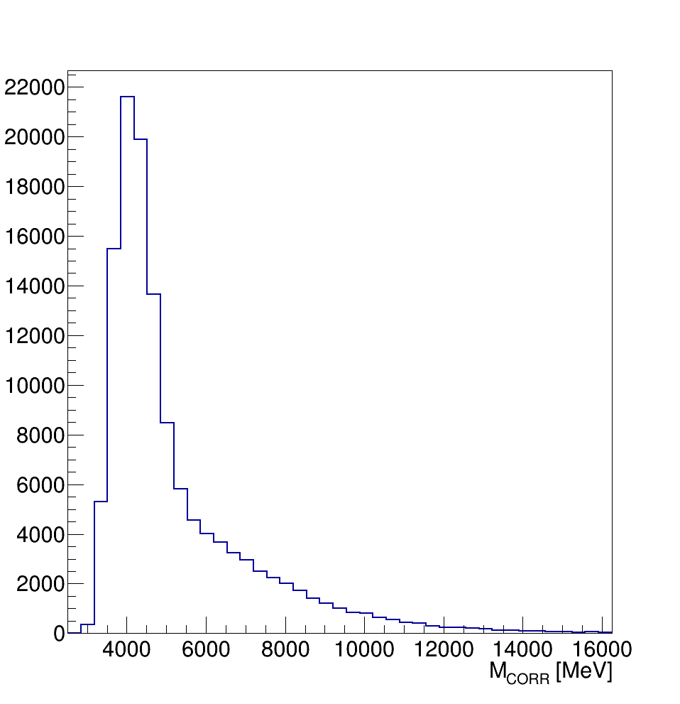
\(M_{CORR}\) resolution study
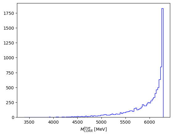
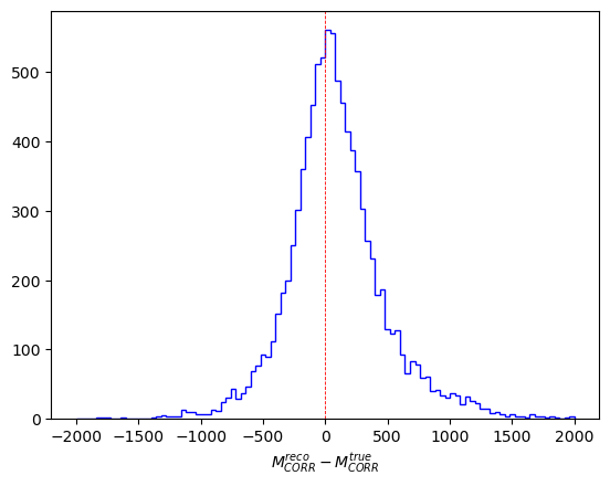
Previous to the signal extraction, it is necessary to check the resolution in the \(M_{CORR}\) using signal MC .
\boxed{\sigma = 397 \pm 3}
Efficiency ratio computation
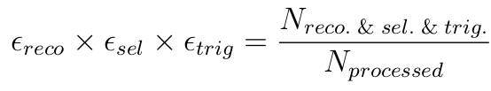
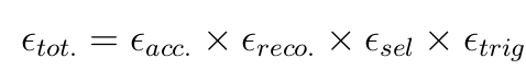
Acceptance efficiency \(\epsilon_{acc}\) from generator-level simulations. The product \(\epsilon_{reco} \times \epsilon_{sel} \times \epsilon_{trig}\) can be calculated as follows:
\(\longrightarrow N_{processed} = 1\)M events
Total efficiency
S. Ordonez Soto
June 27th, 2024
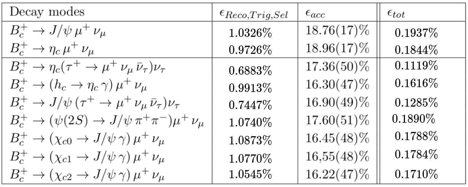
Decay modes efficiency
Efficiency ratio computation
S. Ordonez Soto
June 27th, 2024
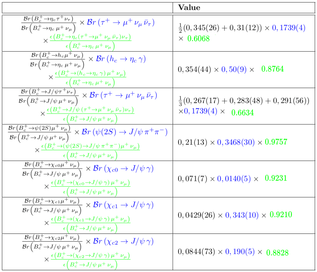
The yields of the peaking background decays are fixed with respect to the yields of the signal with the values shown in the table:
LHCb IJCLab internship presentation: Bc2etacmunu
By Sebastian Ordoñez


