S. Akar, E. Cogneras, S. Monteil, S. Ordonez-Soto*
B2KShh' \(\mu\)-group Meeting
April 14th, 2025


Time-integrated Amplitude Analysis of the decay \(B_{s}\rightarrow K_{S}^{0}\pi^{+}\pi^{-}\) with Run I and Run II data
Outline
Sebastian Ordoñez-Soto
April 14th, 2025
- Introduction
- Analysis strategy
-
Towards the nominal DP model
- Mass fit
- Efficiency maps
- Background model
- Preliminary Dalitz plot fit
- Conclusion and outlook
AmAn of the \(B_{s}^{0}\rightarrow K_{S}^{0} \pi^{+}\pi^{-}\) decay
Introduction
AmAn of the \(B_{s}^{0}\rightarrow K_{S}^{0} \pi^{+}\pi^{-}\) decay
Sebastian Ordoñez-Soto
April 14th, 2025
Introduction
Sebastian Ordoñez-Soto
AmAn of the \(B_{s}^{0}\rightarrow K_{S}^{0} \pi^{+}\pi^{-}\) decay
April 14th, 2025
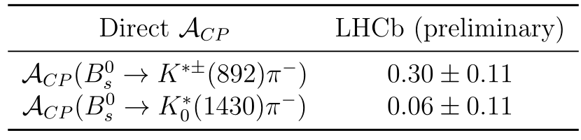
- The Amplitude Analysis of the \(B_{s}^{0}\rightarrow K_{S}^{0}\pi^{+}\pi^{-}\) provides access to the following observables:
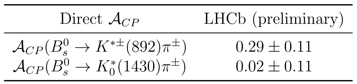
- The direct \(CP\) asymmetries of the quasi-two-body decays with an untagged time-integrated (TI) Dalitz analysis:
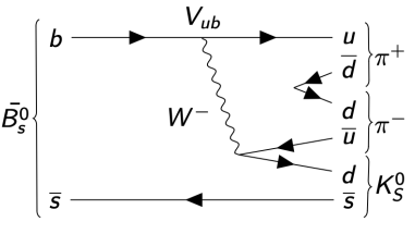
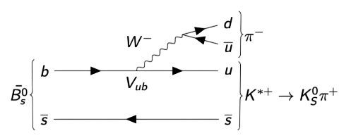
- Flavour specific: \(\bar{B}_{s}^{0}\rightarrow K^{*+}_{0}(1430)\pi^{-}\), \(\bar{B}_{s}^{0}\rightarrow K^{*+}(892)\pi^{-}\)
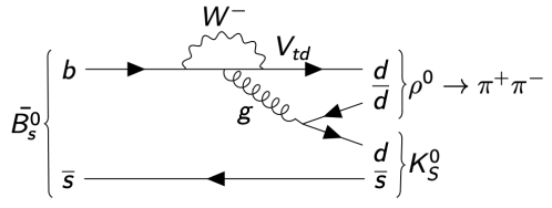
- \(CP\)-eigenstates: \(B_{s}^{0}\rightarrow \rho^{0}K_{S}^{0}\)
- Fit fractions of the different amplitudes contributing to the decay.
- The direct \(CP\) asymmetries of the quasi-two-body decays with an untagged time-integrated (TI) Dalitz analysis:
Physics motivation
Data sample
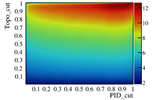
- The data used in this analysis corresponds to: B2pipiKS Secondary Optimization
-
The cut
ProbNNp < 0.9has been included. - Let's recall the charm and charmonia vetoes applied:
- Charm meson vetoes (30 MeV): \(D^{+}_{(s)}\rightarrow K_{S}^{0}\pi^{+}\), \(D^{0}\rightarrow \pi^{+}\pi^{-}\)
- Charmonia vetoes (48 MeV): \(J/\psi\rightarrow \pi^{+}\pi^{-}\), \(\chi_{c0}\rightarrow \pi^{+}\pi^{-}\)
-
The cut
Introduction
Sebastian Ordoñez-Soto
AmAn of the \(B_{s}^{0}\rightarrow K_{S}^{0} \pi^{+}\pi^{-}\) decay
April 14th, 2025
The general PDf describing the dynamics of the decay \(B_{s}^{0}\rightarrow K_{S}^{0}\pi^{+}\pi^{-}\) reads:
Dalitz signal PDF
\mathcal{S}(s_{+},s_{-},t,r_{\text{tag}}) = \frac{\text{d} \Gamma_{B^0_{S},\bar{B}^{0}_{S}}(t)}{\text{d}t} = \frac{ 1}{2}e^{-\Gamma t} \left( |\mathcal{A}(s_{+},s_{-})|^2 + |\bar{\mathcal{A}}(s_{+},s_{-})|^2 \right)\left[ \cosh(\Gamma yt) - K \sinh(\Gamma yt) + r_{\text{tag}}\left(C\cos(\Gamma x t) - S \sin(\Gamma x t)\right)\right]
- \(\mathcal{A}_{f} = \langle f|H_{\Delta F=1}|B_{s}^{0}\rangle\) and \(\bar{\mathcal{A}}_{f} = \langle f|H_{\Delta F=1}|\bar{B}_{s}^{0}\rangle\)
- \(S\), \(C\) and \(K\) are the time-dependent \(CP\) asymmetries
- \(r_{t}\) tagging parameter
- \(\Gamma\) and \(\Delta m\) are the decay rate and mass difference, respectively.
- After integration and with \(r_{\text{tag}} = 0\) simplifies as:
\mathcal{S}(s_{+},s_{-}) \propto |\mathcal{A}(s_{+},s_{-})|^2 + |\bar{\mathcal{A}}(s_{+},s_{-})|^2
- \(\mathcal{A}\) is parametereized by the isobar model:
|\mathcal{A}(s_+, s_-) |^2 = \left| \sum_j a_j e^{i\phi_j} F_j(s_+, s_-) \right|^2
- \(a_{j}\) and \(\phi_{j}\) describe the relative magnitude and phase.
Analysis Strategy
AmAn of the \(B_{s}^{0}\rightarrow K_{S}^{0} \pi^{+}\pi^{-}\) decay
Sebastian Ordoñez-Soto
April 14th, 2025
Analysis Strategy
Sebastian Ordoñez-Soto
AmAn of the \(B_{s}^{0}\rightarrow K_{S}^{0} \pi^{+}\pi^{-}\) decay
April 14th, 2025
This analysis follows a similar strategy to that of the DP analysis of the decay \(B_{d}^{0}\rightarrow K_{S}^{0}\pi^{+}\pi^{-}\) with Run I data.
- The results were obtained with CRAFT (Clermont Roofit-based Amplitude Fitter Tool).
- Analysis note: ANAnote Run I B02KSpipi
- WG database: Analysis Run I B02KSpipi TI Dalitz Analysis
- Selection of \(B_{s}^{0}\rightarrow K_{S}^{0}\pi^{+}\pi^{-}\) signal candidates
- Fit the mass spectrum \(K_{S}^{0}\pi^{+}\pi^{-}\) and define a signal window around \(B_{s}^{0}\) signal peak.
- Determine the fraction of signal and bkg. (Combinatorial and \(B_{d}^{0}\rightarrow K_{S}^{0}\pi^{+}\pi^{-}\))
- Obtain the spline histogram of the efficiency variation across the DP from MC.
- Determine a model for the different background components.
- Fit simultaneously the different samples an educate the final model.
Precedents
Stages
Analysis Strategy
Sebastian Ordoñez-Soto
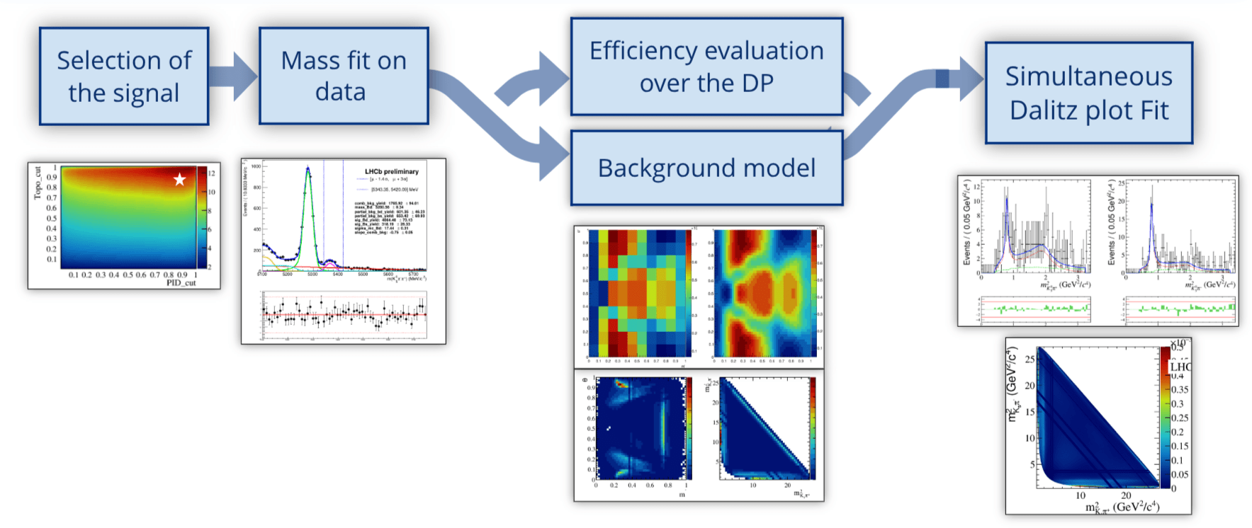
| Selection of the signal |
| Efficiency evaluation over the DP |
| Background model |
| Simultaneous Dalitz plot Fit |
| Mass fit on data |
Schematic of the analysis workflow
AmAn of the \(B_{s}^{0}\rightarrow K_{S}^{0} \pi^{+}\pi^{-}\) decay
April 14th, 2025

Sebastian Ordoñez-Soto
AmAn of the \(B_{s}^{0}\rightarrow K_{S}^{0} \pi^{+}\pi^{-}\) decay
Analysis Strategy

Done!
Inherited from the BF Analysis
April 14th, 2025
Sebastian Ordoñez-Soto
AmAn of the \(B_{s}^{0}\rightarrow K_{S}^{0} \pi^{+}\pi^{-}\) decay
Analysis Strategy
Done?
Pending latest version from the simultaneous fit.
April 14th, 2025
Sebastian Ordoñez-Soto
AmAn of the \(B_{s}^{0}\rightarrow K_{S}^{0} \pi^{+}\pi^{-}\) decay
Analysis Strategy
Efficiency maps available, also inherited from BF analysis.
Done!
March 24th, 2025
Sebastian Ordoñez-Soto
AmAn of the \(B_{s}^{0}\rightarrow K_{S}^{0} \pi^{+}\pi^{-}\) decay
Analysis Strategy
Work in progress!
First fit with a simple model.
April 14th, 2025
Towards the nominal DP model
AmAn of the \(B_{s}^{0}\rightarrow K_{S}^{0} \pi^{+}\pi^{-}\) decay
Sebastian Ordoñez-Soto
April 14th, 2025
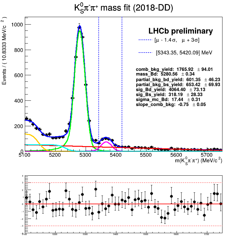
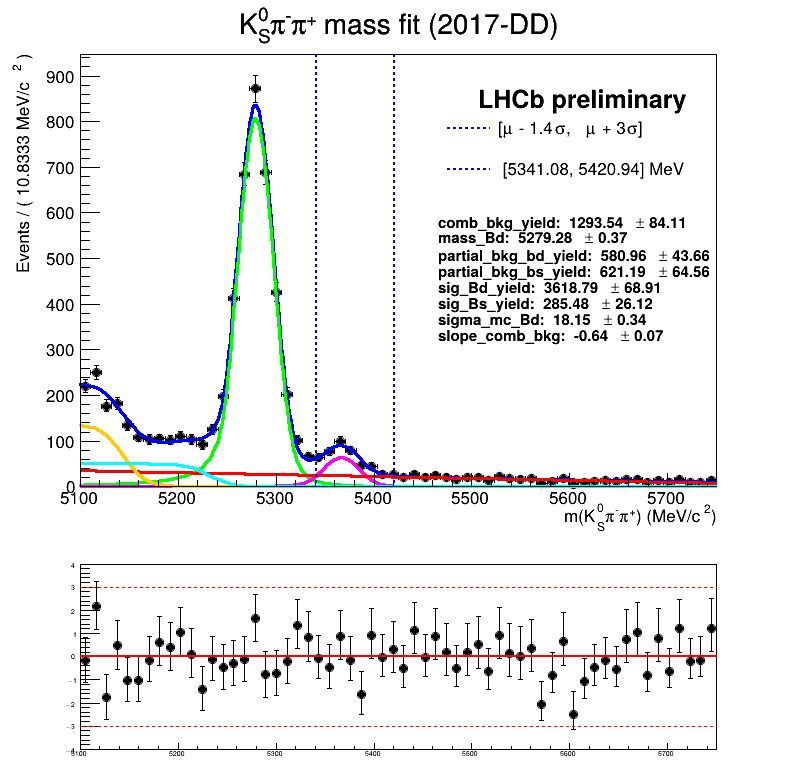
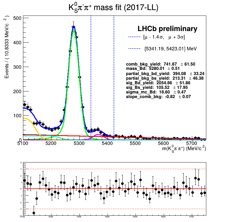
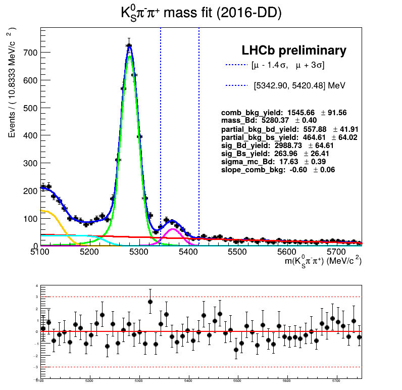
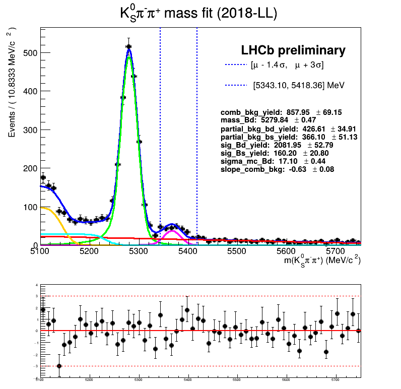
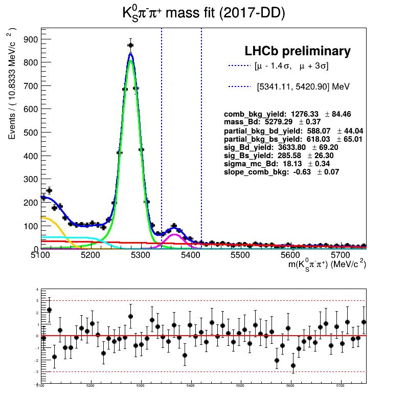
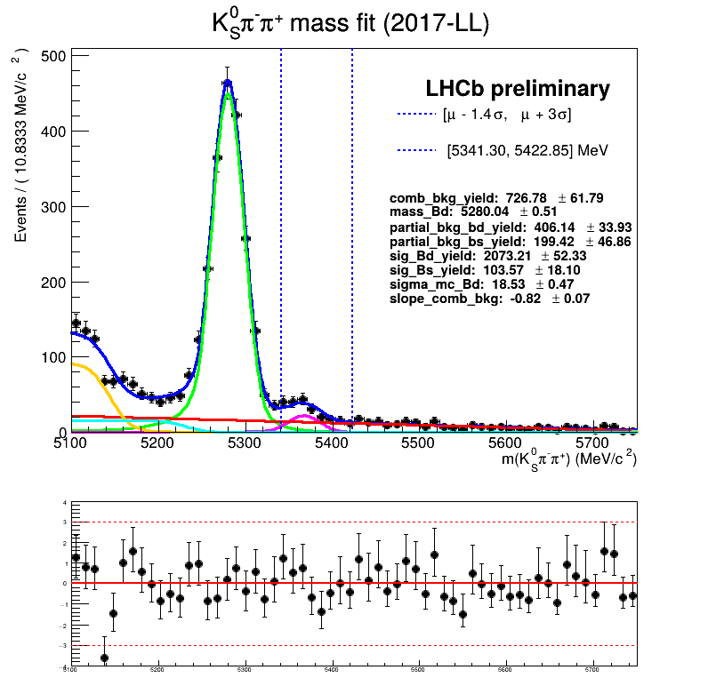
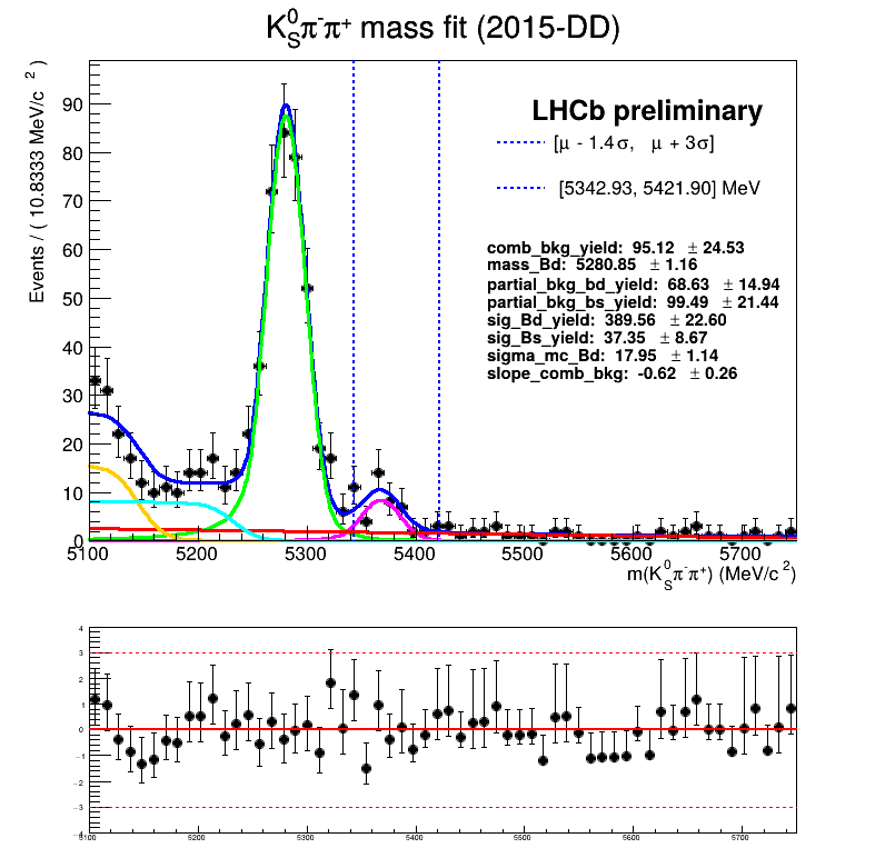
\(K_{S}^{0}\pi^{+}\pi^{-}\) Invariant Mass fit
Sebastian Ordoñez-Soto
AmAn of the \(B_{s}^{0}\rightarrow K_{S}^{0} \pi^{+}\pi^{-}\) decay
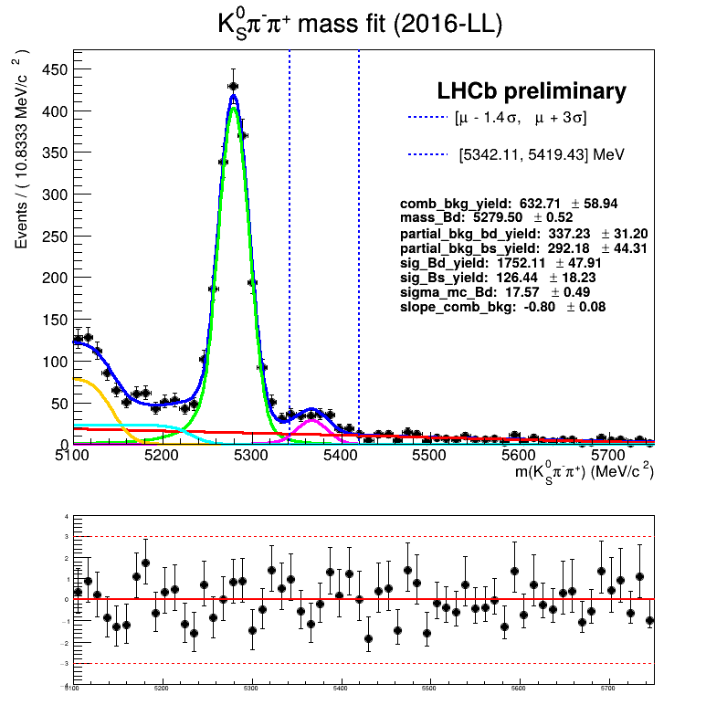
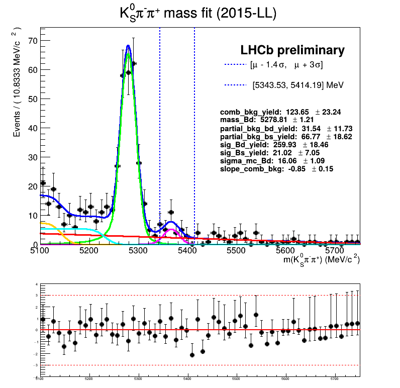
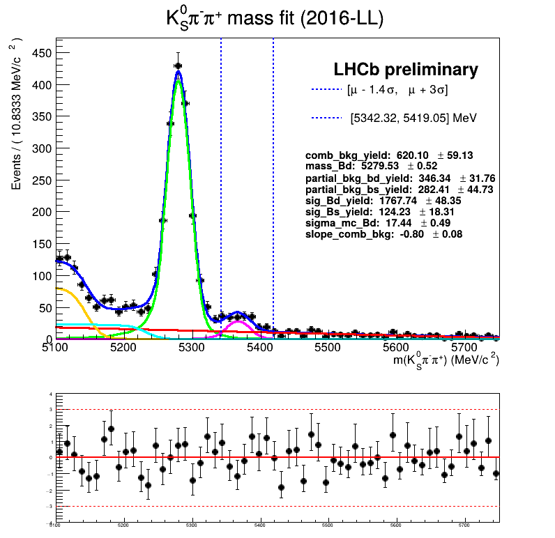
A preliminary fit to the invariant mass, not simultaneous, has been done to determine in the signal mass window (\([\mu_{B_{s}^{0}}-1.4\cdot\sigma_{B_{s}^{0}}, \mu_{B_{s}^{0}}+3.0\cdot\sigma_{B_{s}^{0}}]\)):
- \(f_{\text{sig}}\): Fraction of \(B_{s}^{0}\rightarrow K_{S}^{0}\pi^{+}\pi^{-}\) signal
- \(f_{\text{comb bkg.}}\): Fraction of combinatorial bkg.
- \(f_{B_{d}^{0} \text{ bkg.}}\): Fraction of \(B_{d}^{0}\rightarrow K_{S}^{0}\pi^{+}\pi^{-}\) bkg.
This preliminary fit follows the same procedure than the one of the BF:
- The signal MC, \(B_{s}^{0}\) and \(B_{d}^{0}\), is fitted using a Symmetric Crystal Ball PDF.
- The partial bkg. MC is fitted using: Argus \(\circledast\) Symmetric Crystal Ball PDF.
- The combinatorial bkg. is fitted using a first order polynomial, with the slope floated.
- The shape parameters (\(\alpha_{R,L},n_{R,L}\), etc) are fixed in the data fit.
April 14th, 2025
Sebastian Ordoñez-Soto
AmAn of the \(B_{s}^{0}\rightarrow K_{S}^{0} \pi^{+}\pi^{-}\) decay

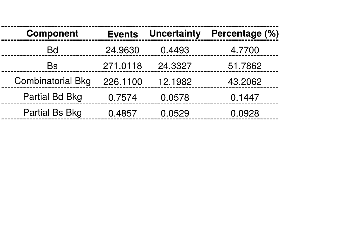
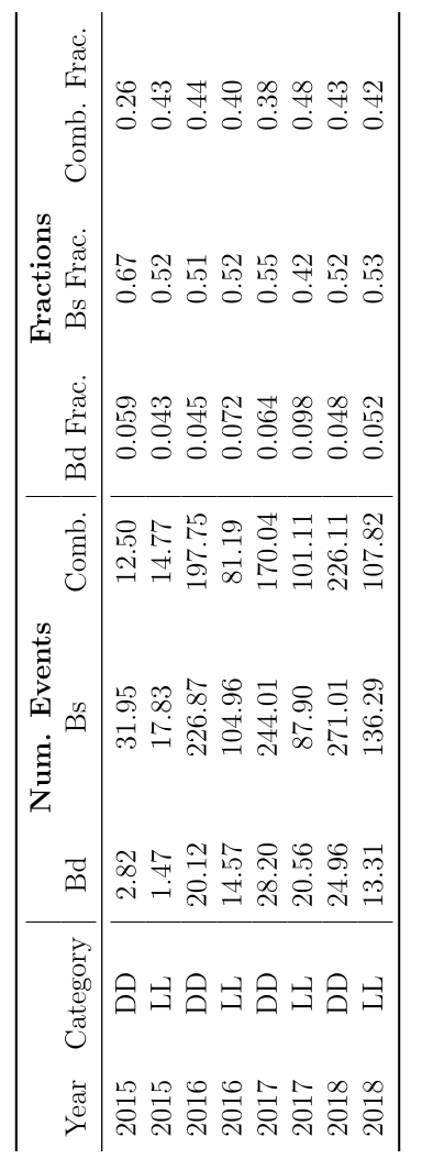
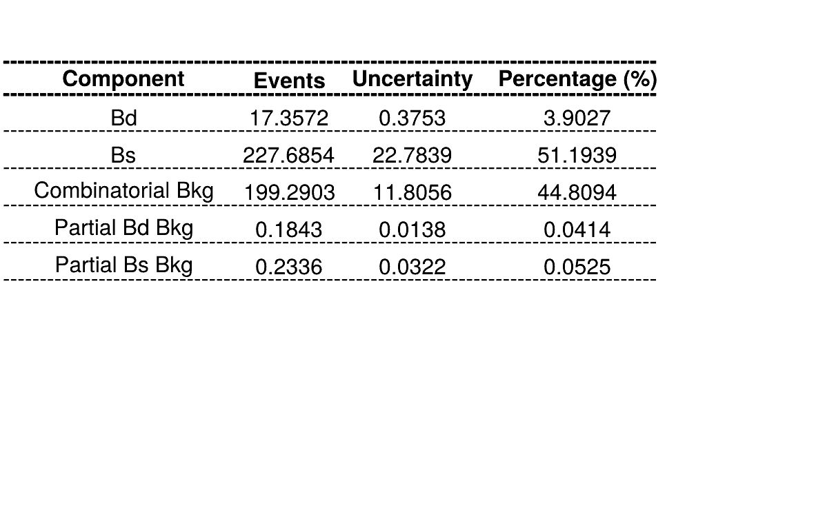
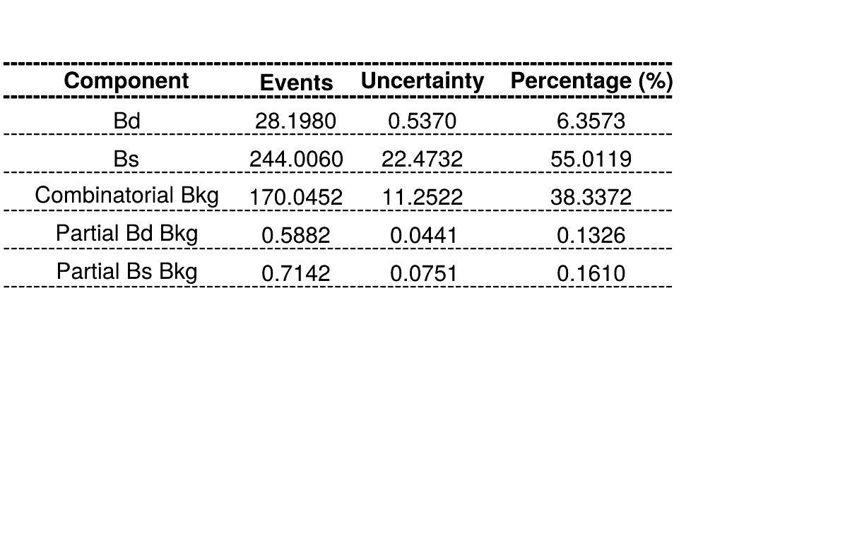
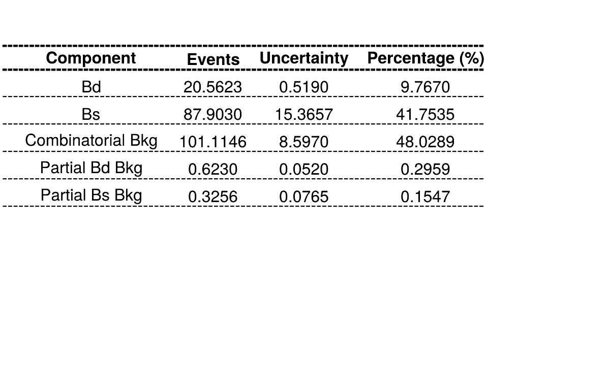
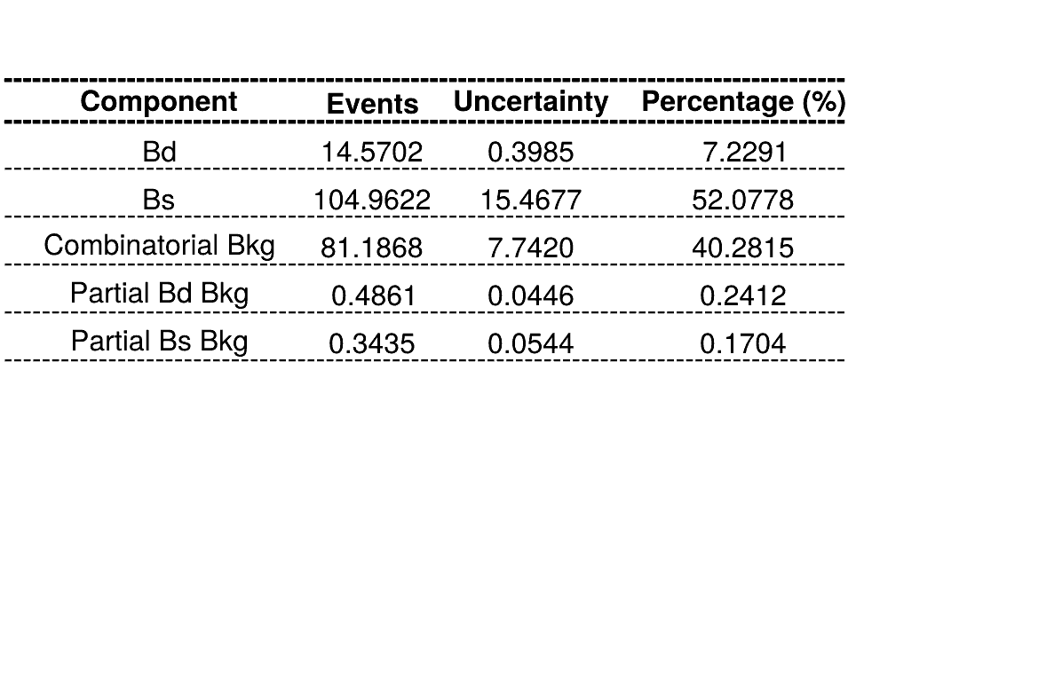
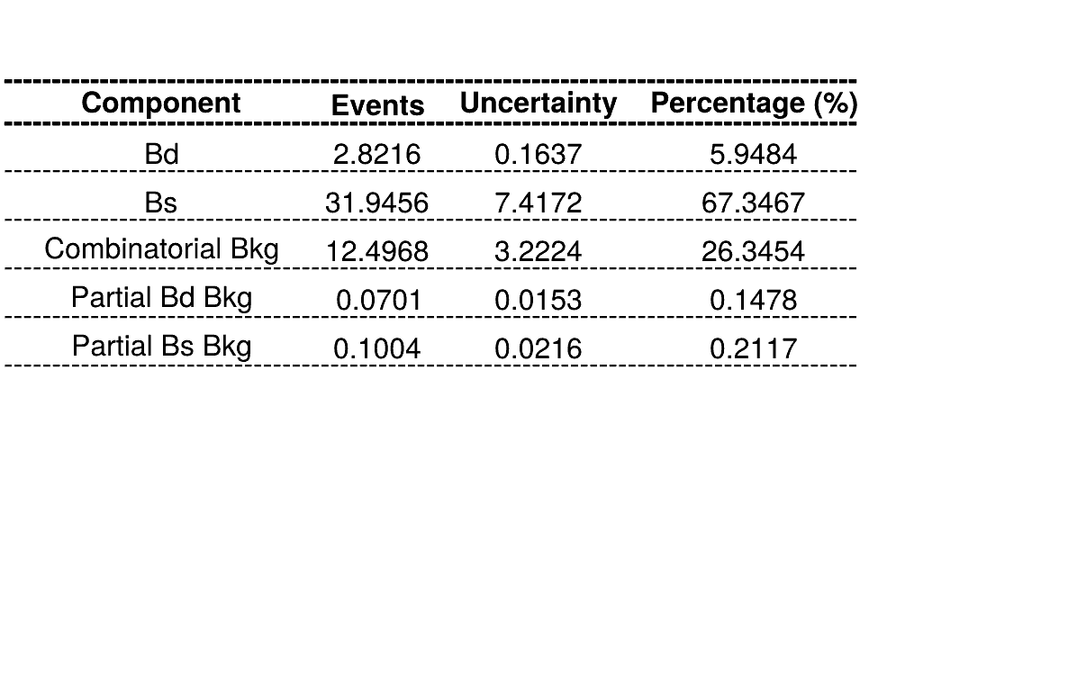
\(K_{S}^{0}\pi^{+}\pi^{-}\) Invariant Mass fit
April 14th, 2025
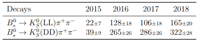
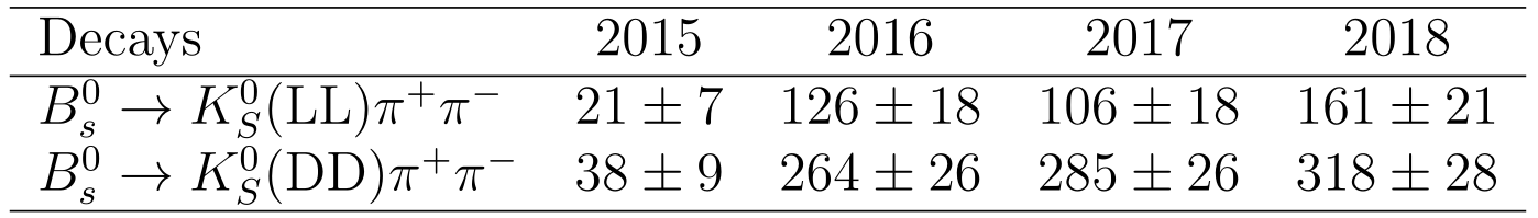
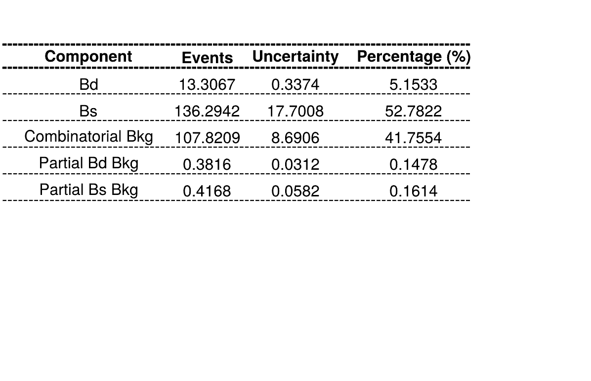
Summary of fractions for each component which are inputs for the Dalitz plot fit.
In the signal window:
- Run 2 DD: \(N_{\text{Sig}}^{B_{s}^{0}} \approx 775 \)
- Run 2 LL: \(N_{\text{Sig}}^{B_{s}^{0}} \approx 345\)
Sebastian Ordoñez-Soto
AmAn of the \(B_{s}^{0}\rightarrow K_{S}^{0} \pi^{+}\pi^{-}\) decay
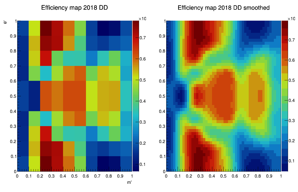
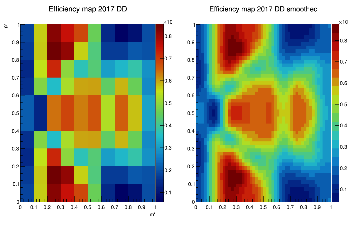
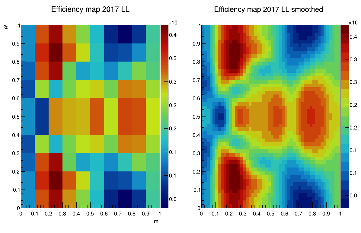
Efficiency across DP
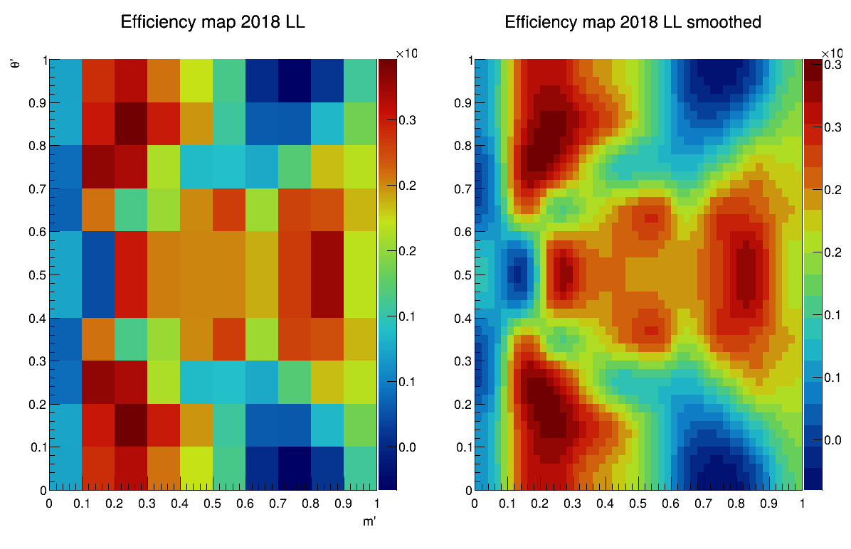
2018-DD
2018-LL
April 14th, 2025
- The efficiency maps in the square Dalitz plot (sDP) have been obtained in the BF analysis.
- For this analysis the spline technique will be the baseline for the efficiency modeling.
- The maps are smoothed out by a 2D cubic spline and are symmetrized.
Sebastian Ordoñez-Soto
AmAn of the \(B_{s}^{0}\rightarrow K_{S}^{0} \pi^{+}\pi^{-}\) decay
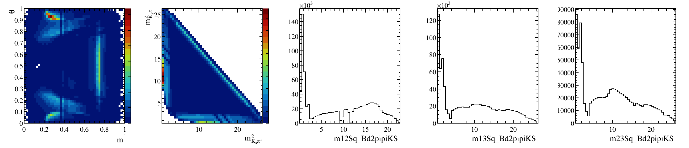
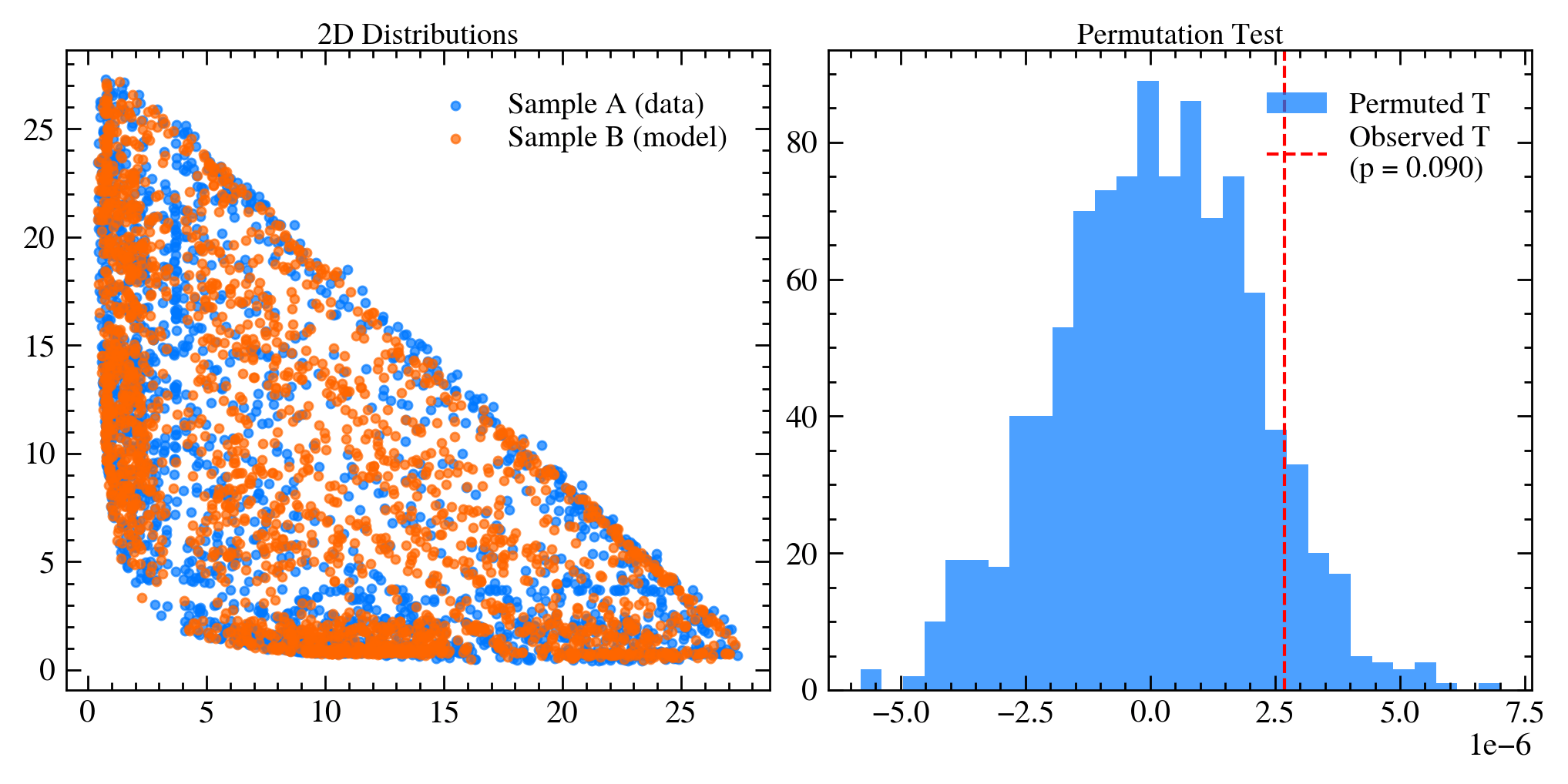
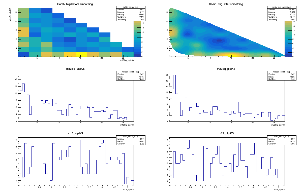
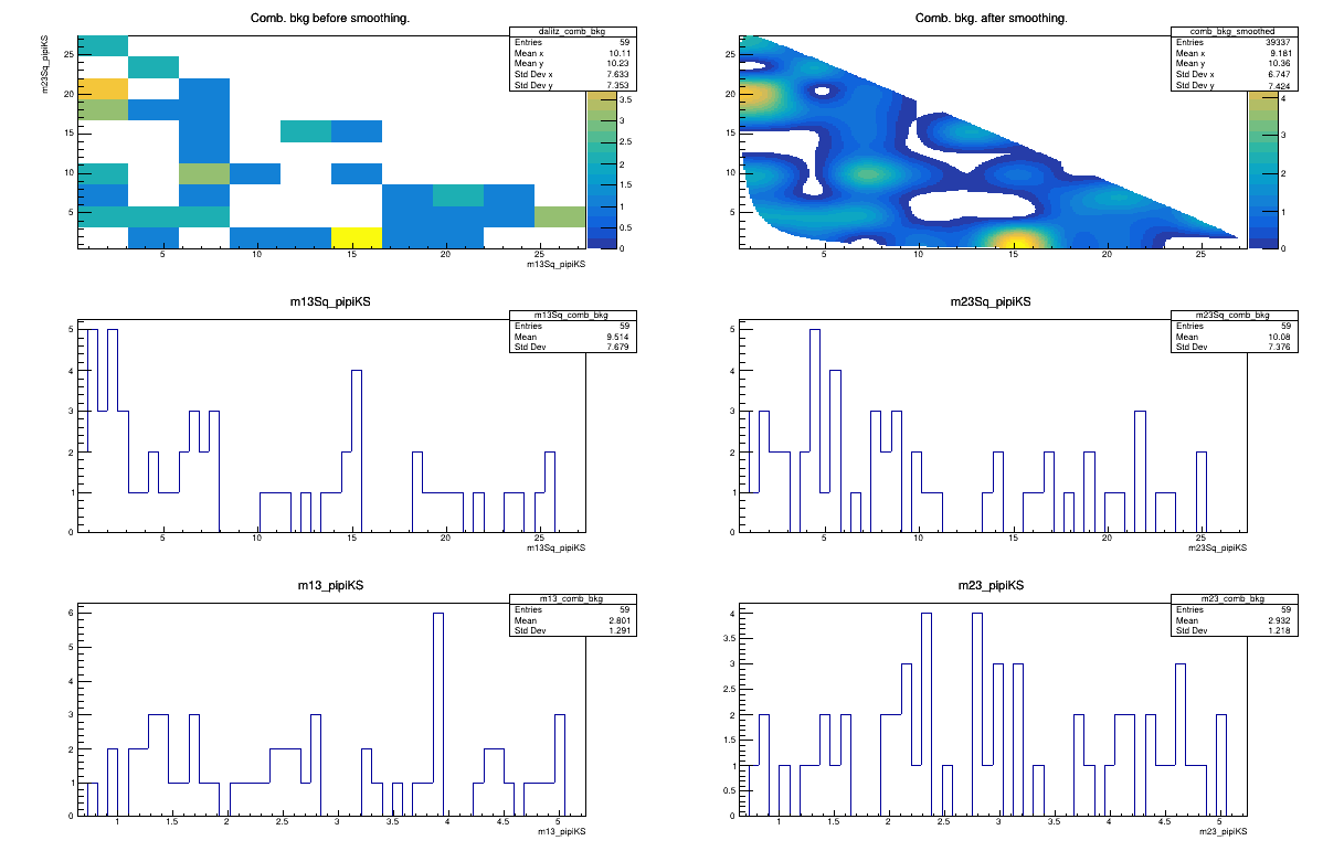
Background model
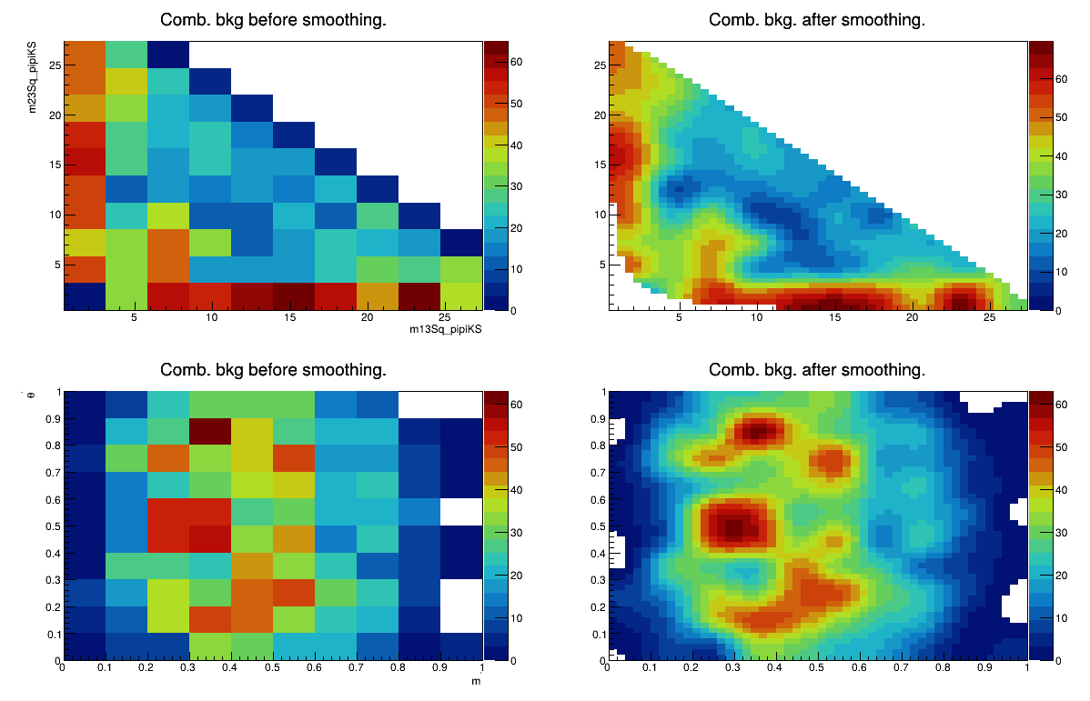
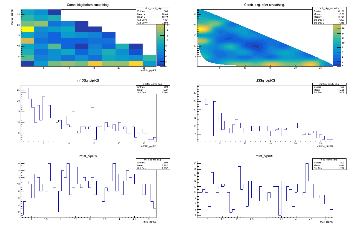
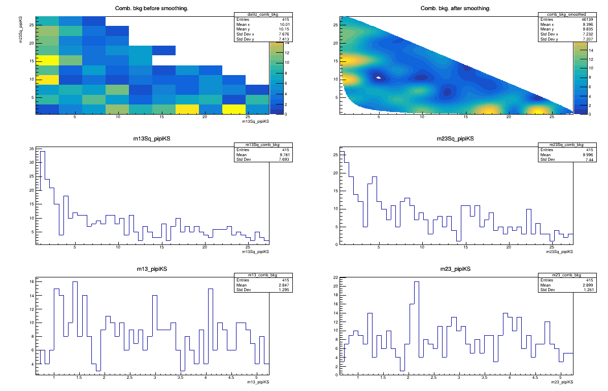
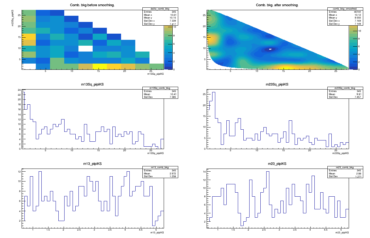
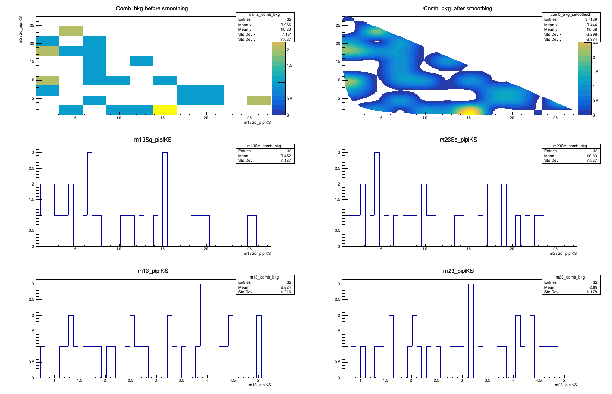
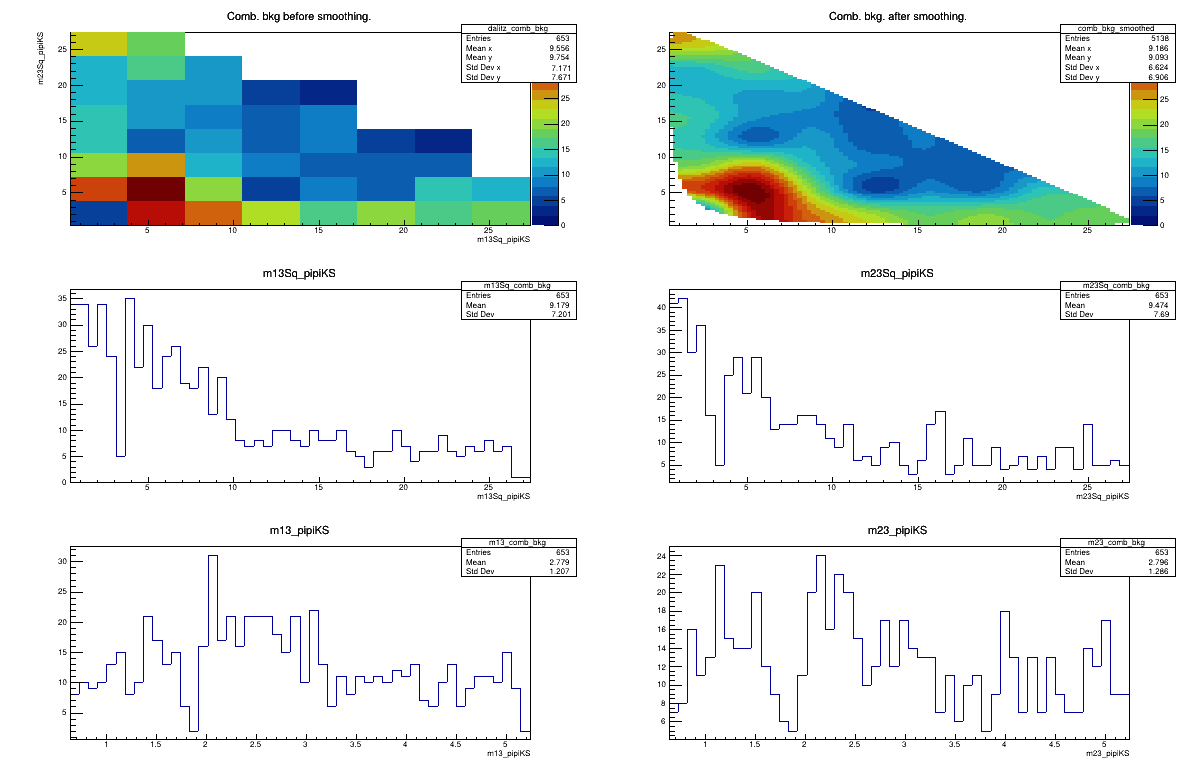
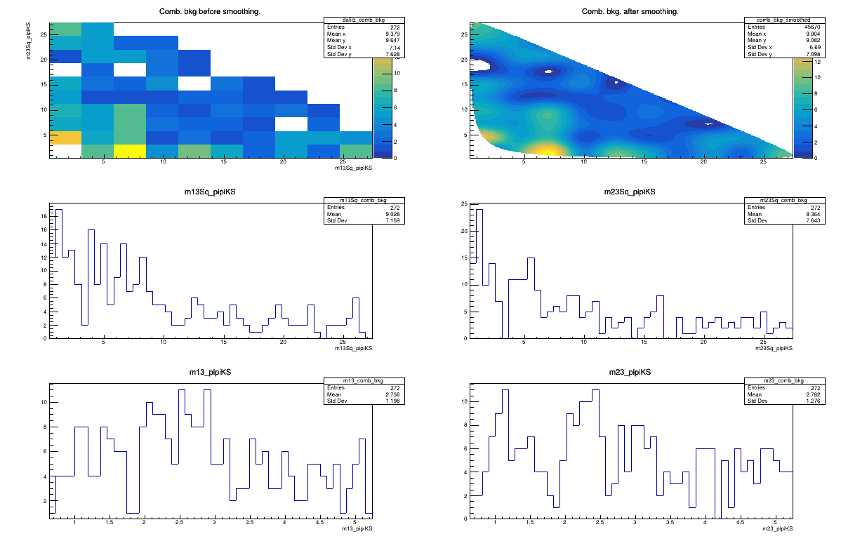
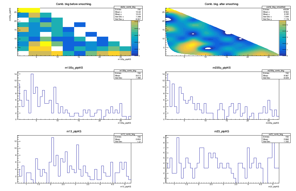
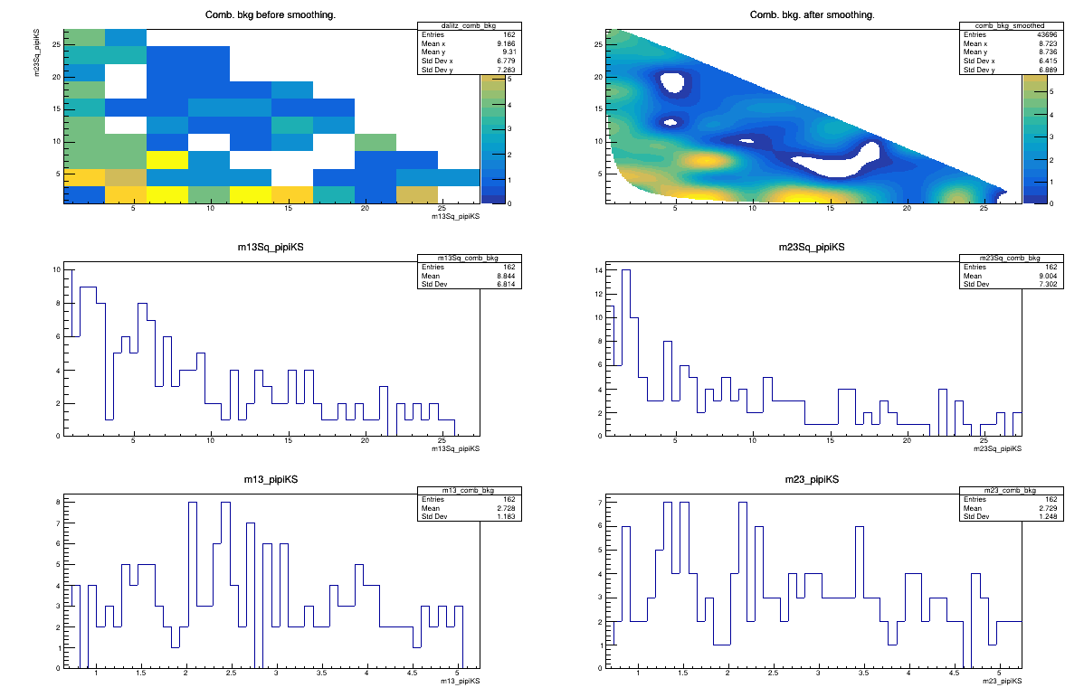
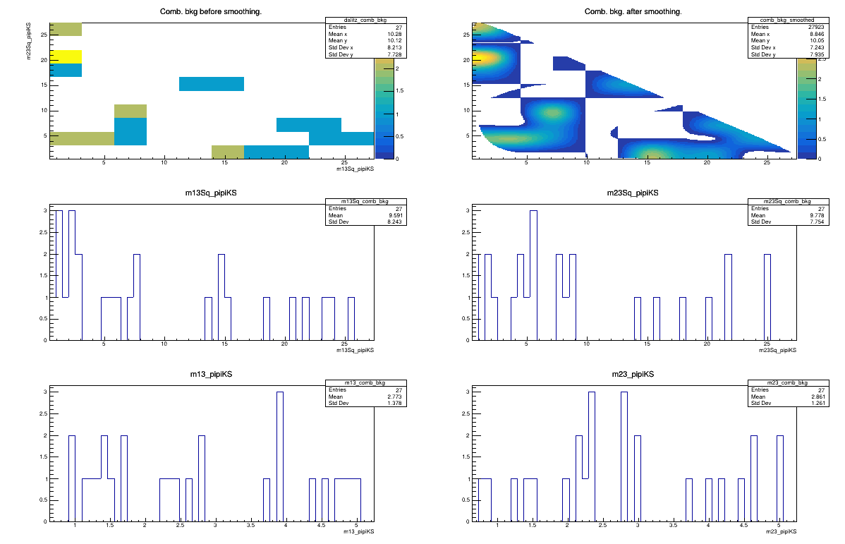
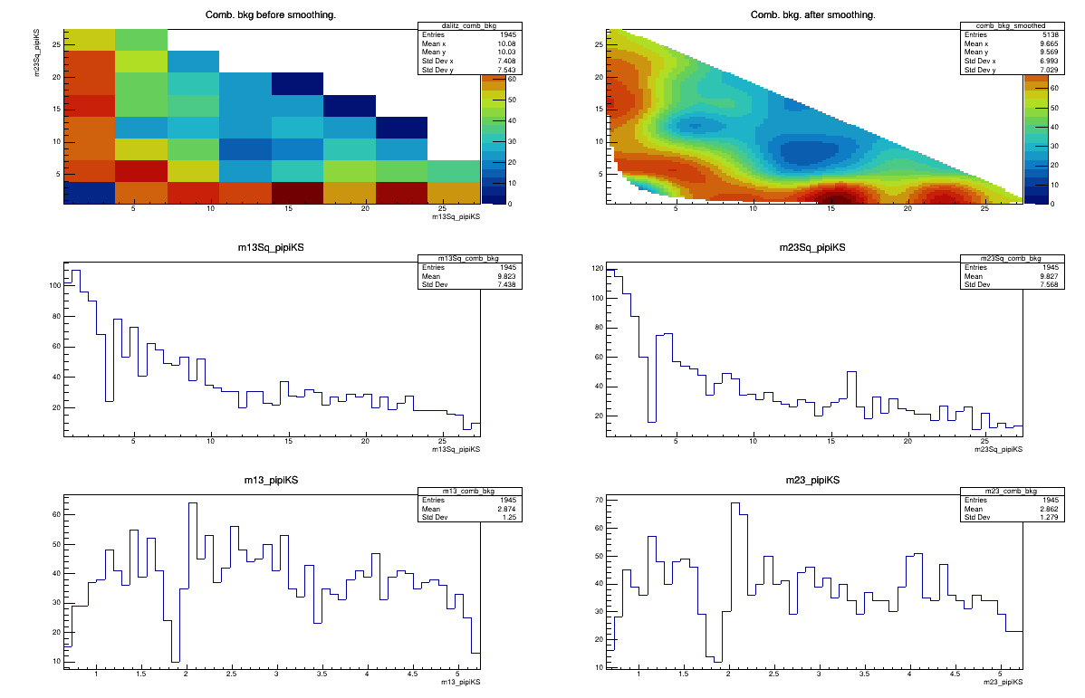
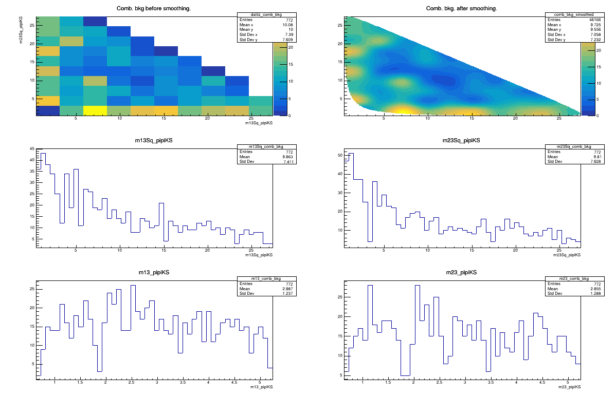
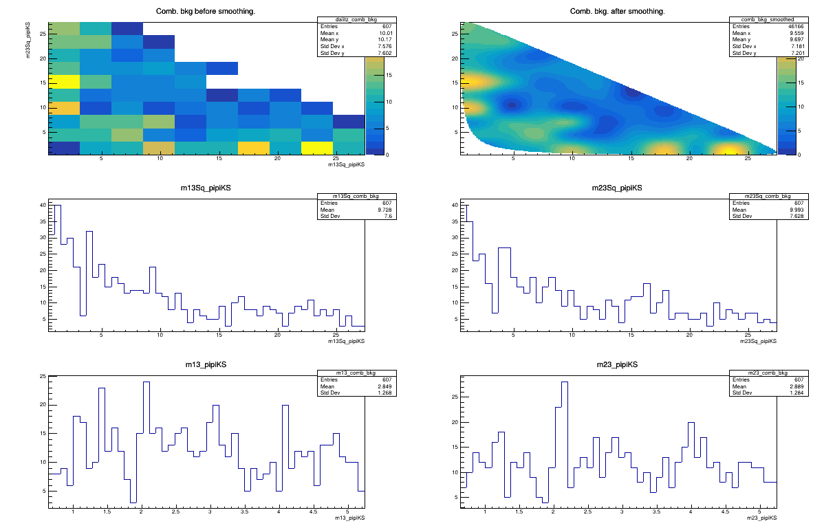
- The combinatorial background under the signal is modeled using candidates from the right-hand sideband
- \([5450,5750] \text{MeV}\)
- Due to the limited statistics, a combined sample including all Run 2 data (DD + LL) is used.
- The resulting background sDP distribution is smoothed and used as input for the combinatorial background model.
April 14th, 2025
Combinatorial background
Sebastian Ordoñez-Soto
AmAn of the \(B_{s}^{0}\rightarrow K_{S}^{0} \pi^{+}\pi^{-}\) decay
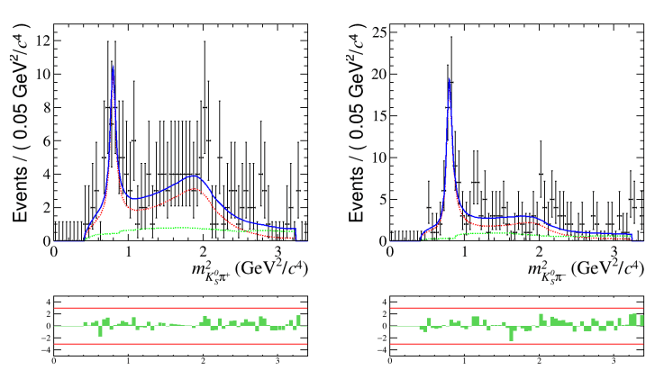
Background model
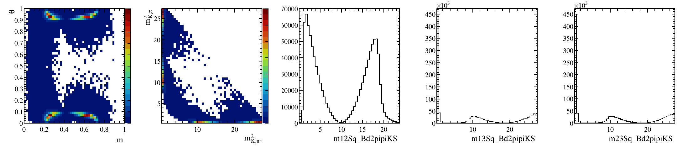
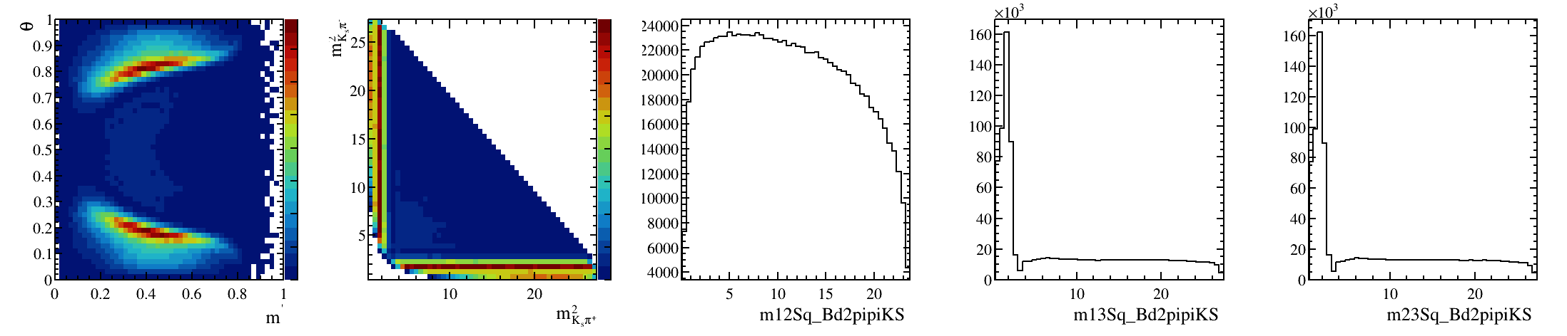
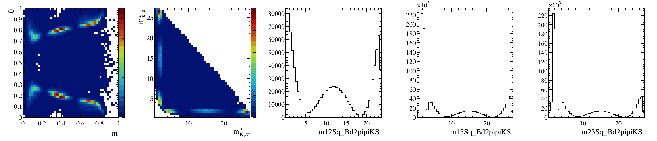
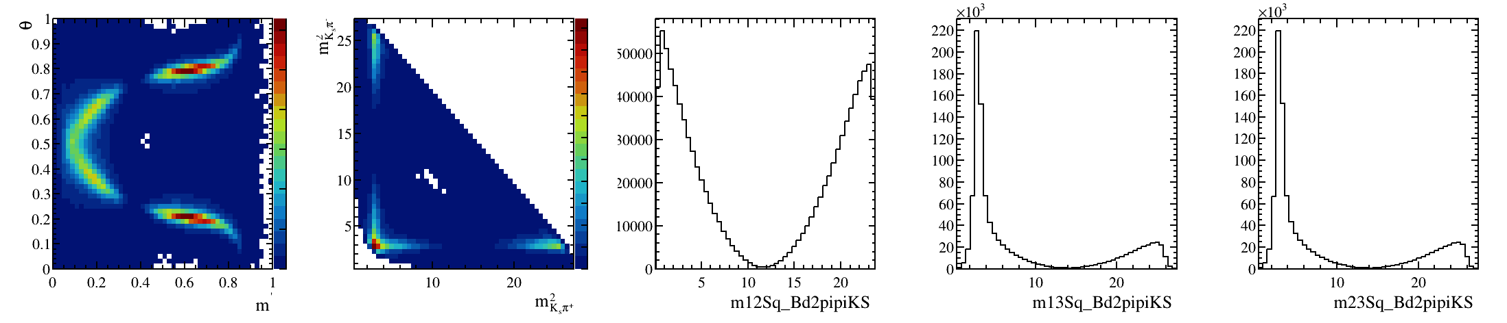
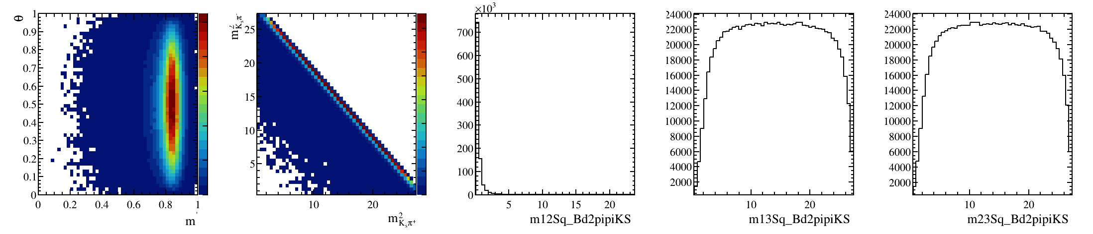
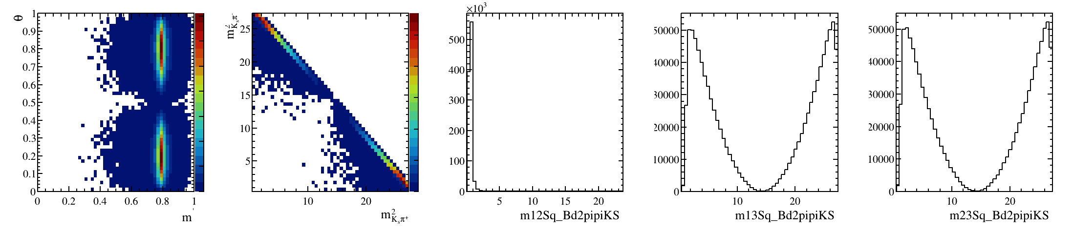
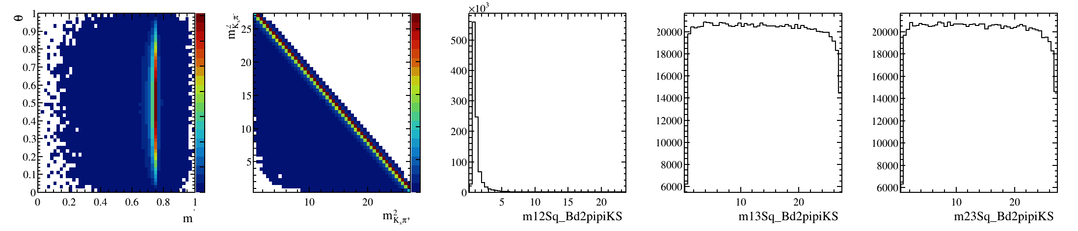
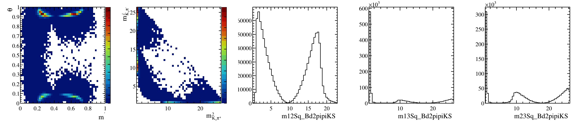
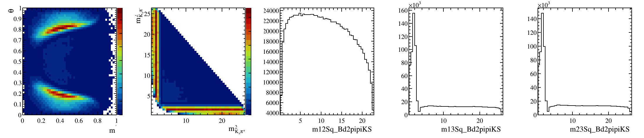
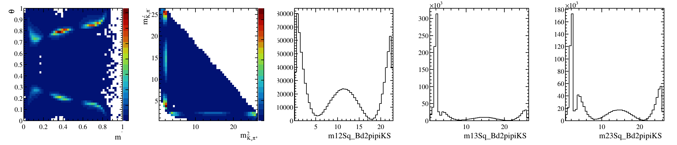
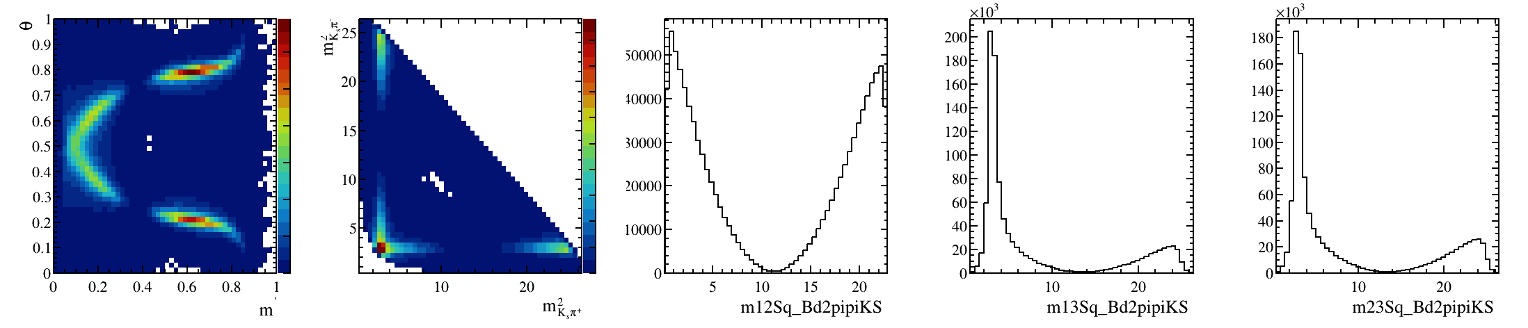
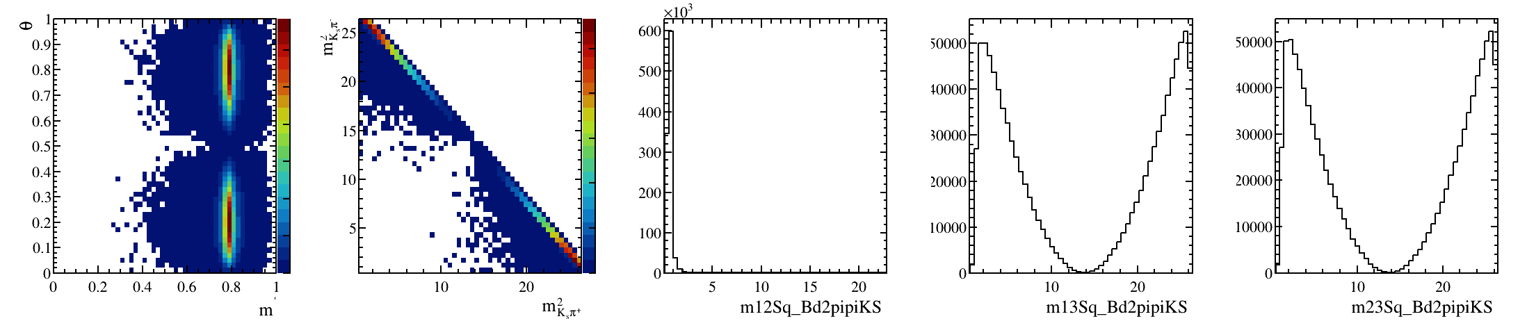
\(B_{d}^{0}\rightarrow K_{S}^{0}\pi^{+}\pi^{-}\) background
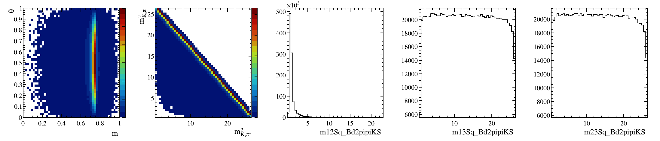
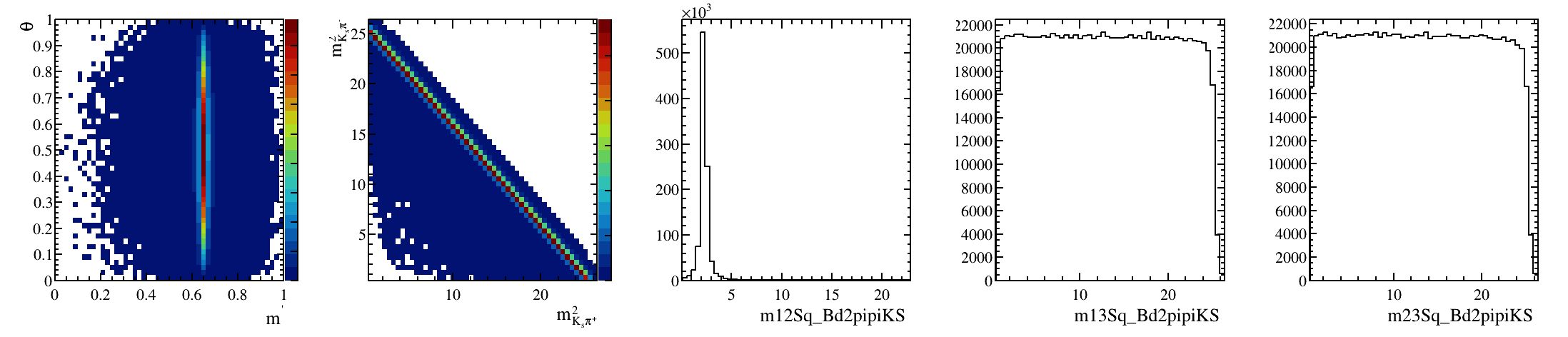
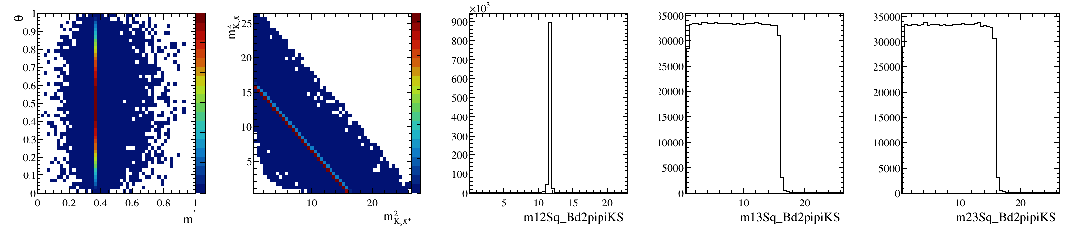
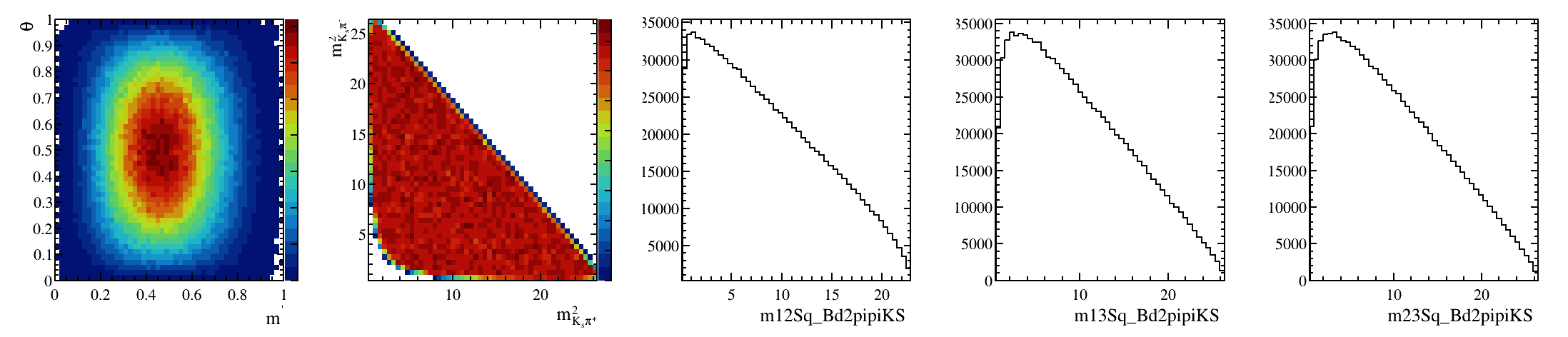
- The \(B_{d}^{0}\rightarrow K_{S}^{0}\pi^{+}\pi^{-}\) background is estimated using the model for this decay from Run I:
- Paper: Amplitude analysis of the decay \(B_{d}^{0}\rightarrow K_{S}^{0}\pi^{+}\pi^{-}\) and first observation of the CP asymmetry in \(B_{d}^{0}\rightarrow K^{*}(892)\pi^{+}\).
- Large toy MC generated using CRAFT.
- The toy MC is weighted by the corresponding efficiency map.
2018-DD
April 14th, 2025
Sebastian Ordoñez-Soto
AmAn of the \(B_{s}^{0}\rightarrow K_{S}^{0} \pi^{+}\pi^{-}\) decay
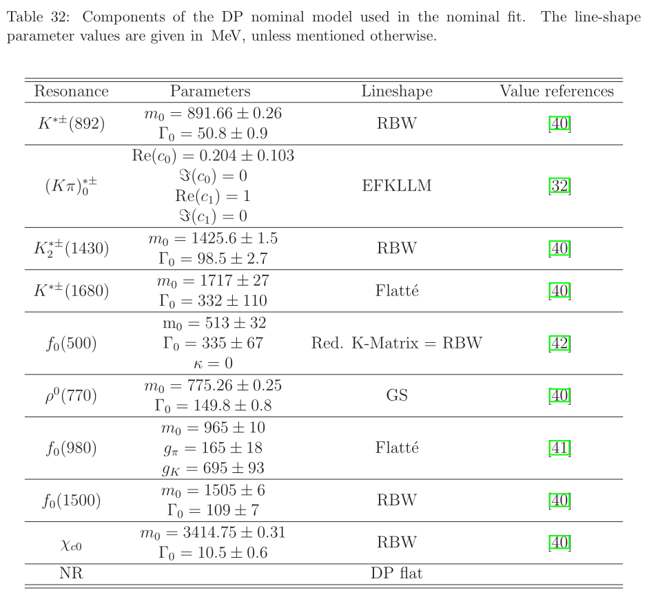
Preliminary signal model
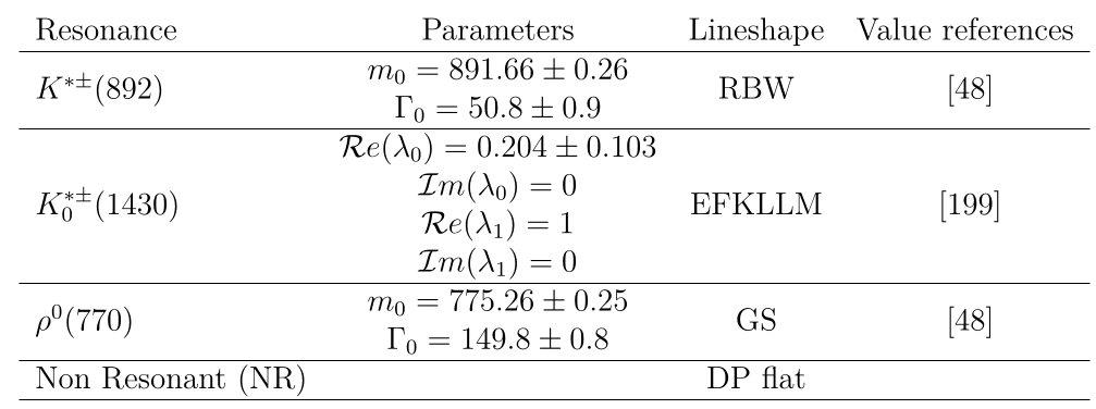
April 14th, 2025
- A preliminary signal model is proposed based on Standard Model expectations.
- \(\overline{B}_s \to \rho^0 K^0_S\)
- \(\overline{B}_s \to K_0^{*+}(1430)\pi^{-}\)
- \(\overline{B}_s \to K^0_S \pi^+ \pi^- \text{ (NR)}\)
- \(\overline{B}_s \to K^{*+}(892) \pi^-\)
- The model parameterizes the signal amplitude as the isobar sum of three resonances (and conjugates) plus a non-resonant (NR) contribution.
*Chosen as reference \(\Rightarrow\) \(x=2\), \(y=0\) and \(\bar{y} = 0\)
*
Dalitz Plot fitting
AmAn of the \(B_{s}^{0}\rightarrow K_{S}^{0} \pi^{+}\pi^{-}\) decay
Sebastian Ordoñez-Soto
April 14th, 2025
Sebastian Ordoñez-Soto
AmAn of the \(B_{s}^{0}\rightarrow K_{S}^{0} \pi^{+}\pi^{-}\) decay
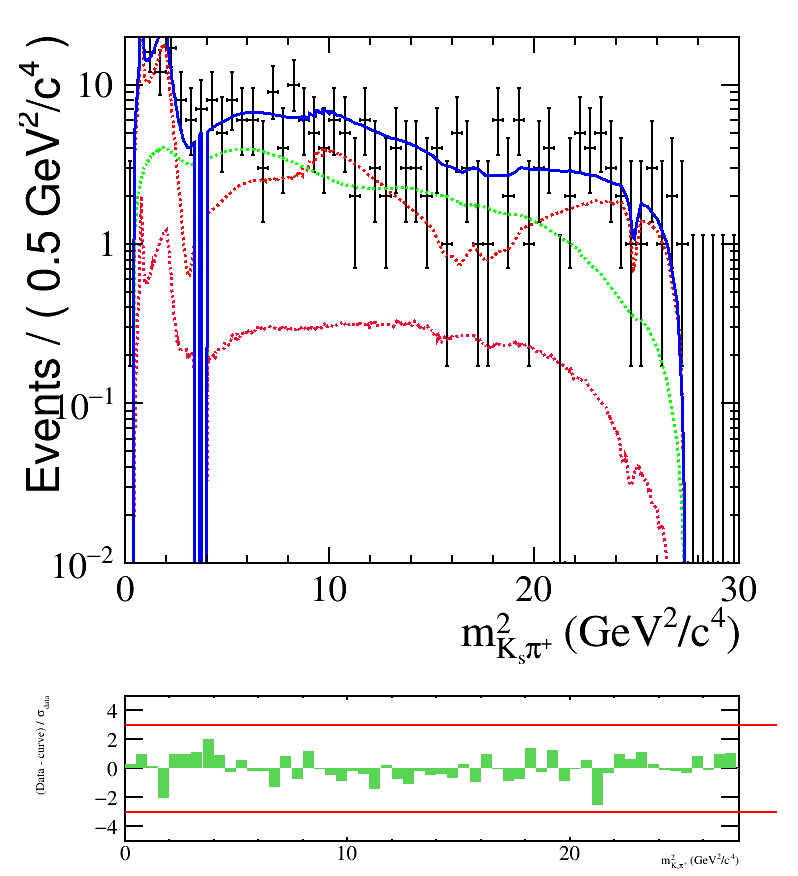
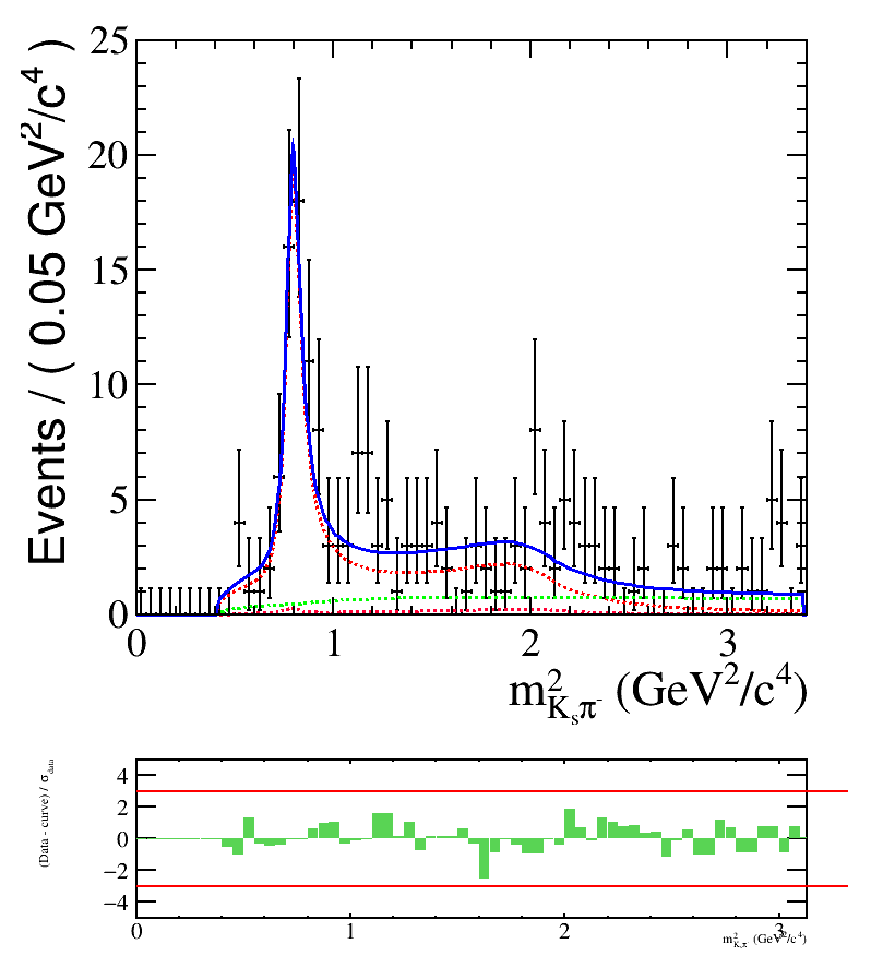
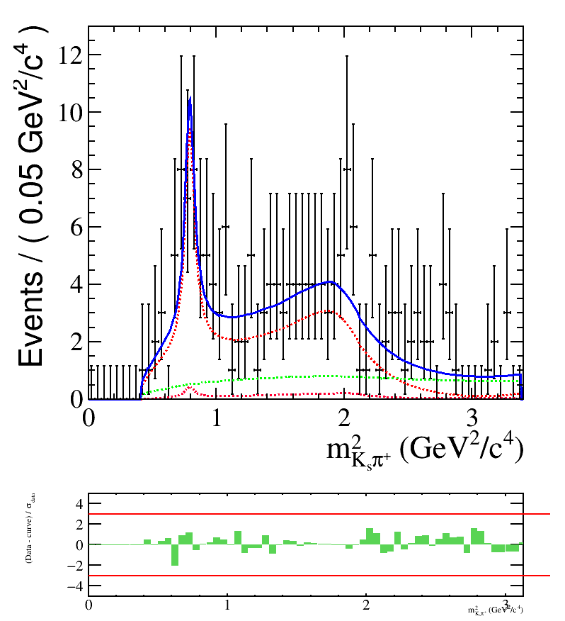
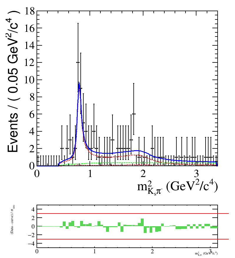
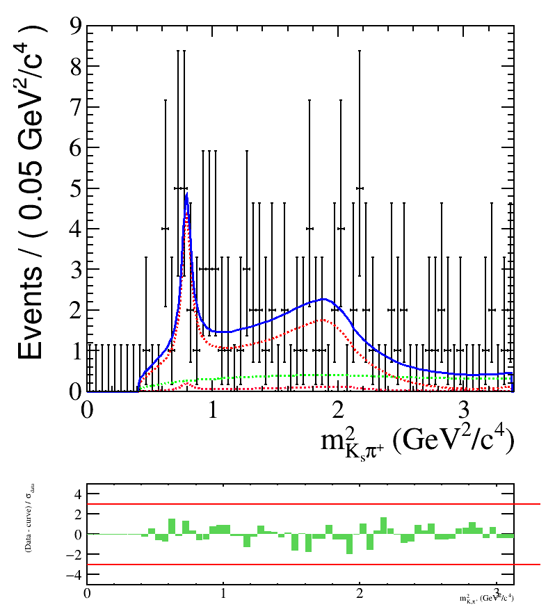
Dalitz plot Fit
- A simultaneous fit to DD+LL 2018 data has been done using the simple signal model.


April 14th, 2025
2018-LL \(\Rightarrow\)
2018-DD \(\Rightarrow\)
Sebastian Ordoñez-Soto
AmAn of the \(B_{s}^{0}\rightarrow K_{S}^{0} \pi^{+}\pi^{-}\) decay
Dalitz plot Fit


April 14th, 2025
2018-LL \(\Rightarrow\)
2018-DD \(\Rightarrow\)
Sebastian Ordoñez-Soto
AmAn of the \(B_{s}^{0}\rightarrow K_{S}^{0} \pi^{+}\pi^{-}\) decay
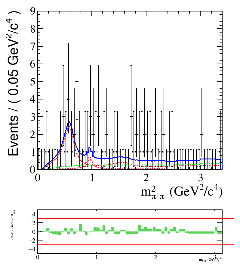
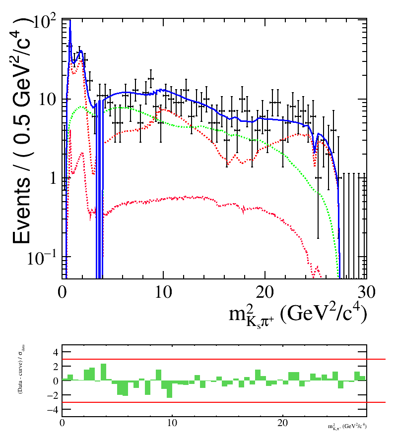
Dalitz plot Fit
April 14th, 2025
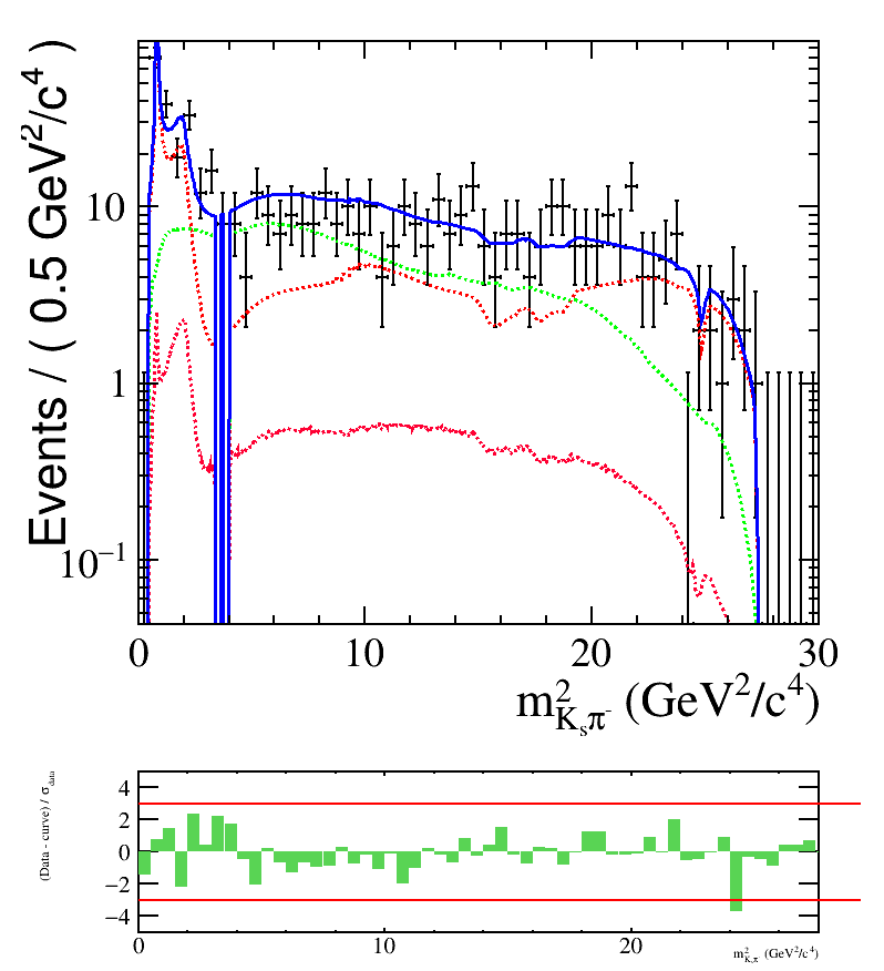
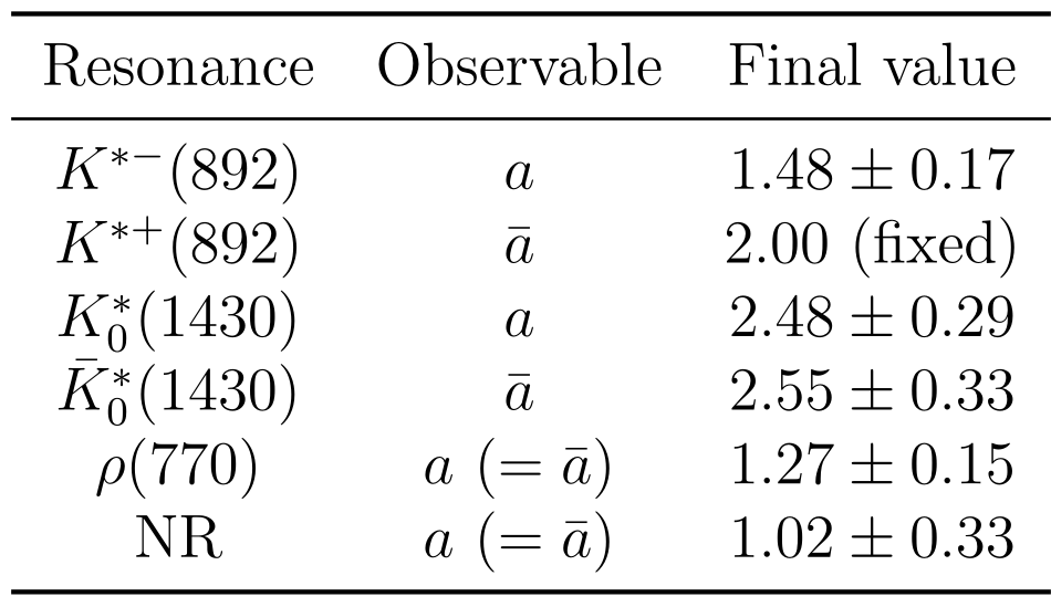
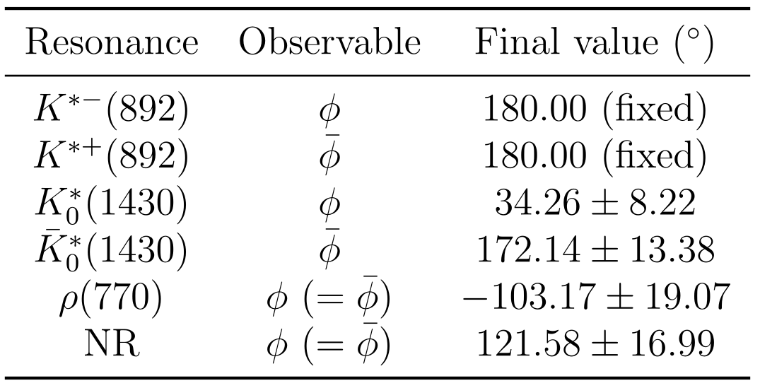
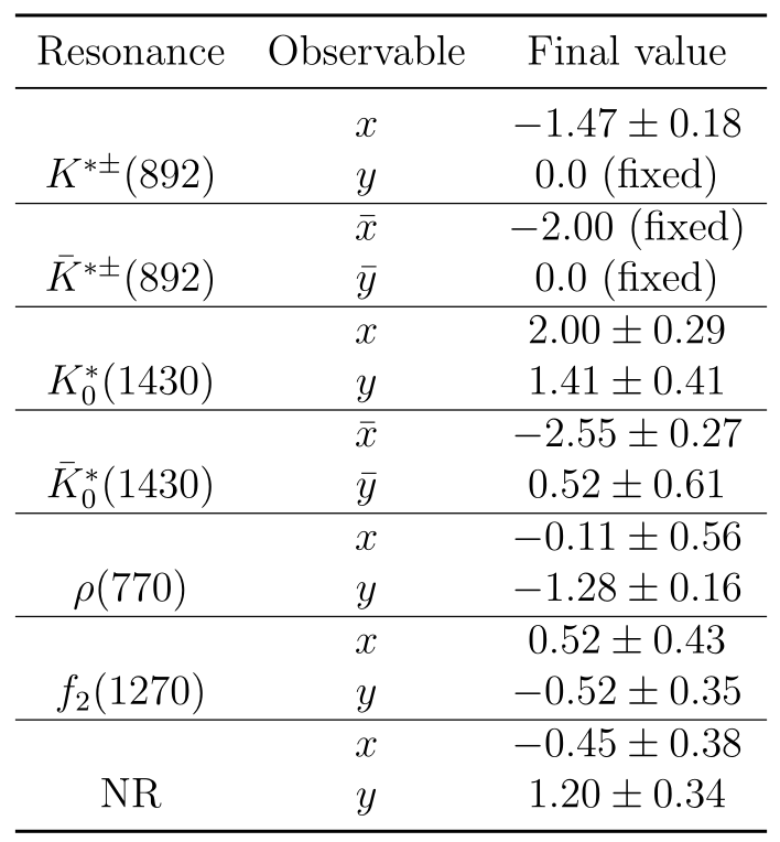
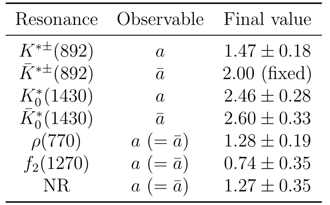
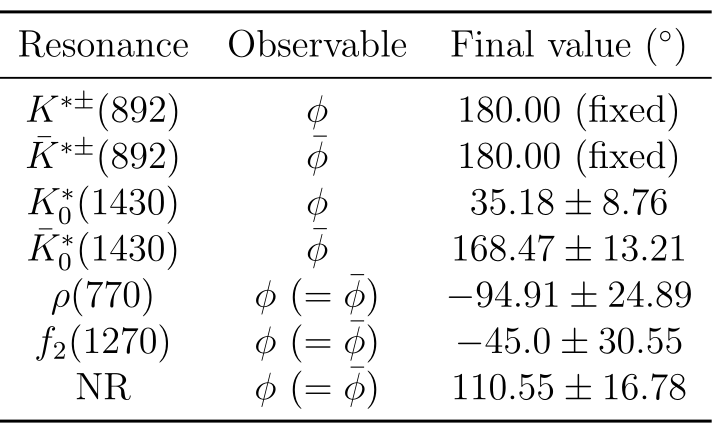
Fit results

- The simple model presents a reasonable description of the Dalitz plot data.
Amplitudes
Phases
Dalitz plot PDF

Sebastian Ordoñez-Soto
AmAn of the \(B_{s}^{0}\rightarrow K_{S}^{0} \pi^{+}\pi^{-}\) decay
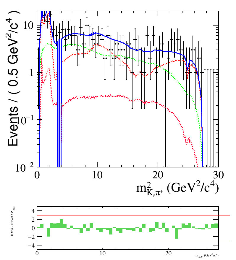
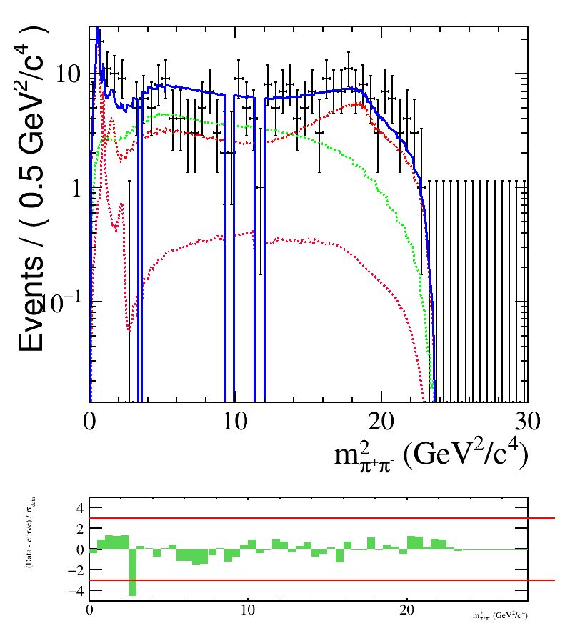
Dalitz plot Fit
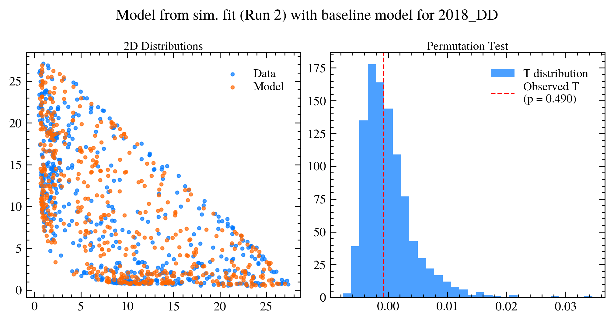
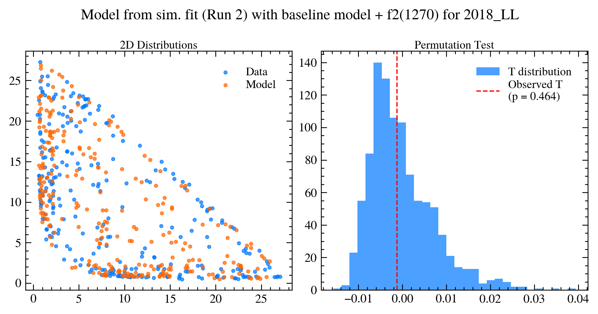
- A simultaneous fit to DD+LL 2018 data has been done using the simple model + \(f_{2}(1270)\).
April 14th, 2025
2018-LL \(\Rightarrow\)
2018-DD \(\Rightarrow\)

Sebastian Ordoñez-Soto
AmAn of the \(B_{s}^{0}\rightarrow K_{S}^{0} \pi^{+}\pi^{-}\) decay
Dalitz plot Fit
April 14th, 2025
2018-LL \(\Rightarrow\)
2018-DD \(\Rightarrow\)


Sebastian Ordoñez-Soto
AmAn of the \(B_{s}^{0}\rightarrow K_{S}^{0} \pi^{+}\pi^{-}\) decay
Dalitz plot Fit
April 14th, 2025
Amplitudes
Phases
Dalitz plot PDF
Fit results
- A simultaneous fit to DD+LL 2018 data has been done using the simple model + \(f_{2}(1270)\).

Conclusion and Outlook
AmAn of the \(B_{s}^{0}\rightarrow K_{S}^{0} \pi^{+}\pi^{-}\) decay
Sebastian Ordoñez-Soto
April 14th, 2025
Sebastian Ordoñez-Soto
AmAn of the \(B_{s}^{0}\rightarrow K_{S}^{0} \pi^{+}\pi^{-}\) decay
Conclusion and outlook
April 14th, 2025
- Most elements for the time integrated Dalitz plot are in place.
- Preliminary simultaneous (only 2018) fit with a simple model gives a reasonable description of the Dalitz for both DD and LL.
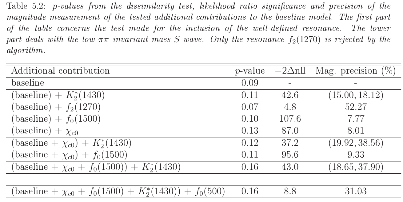
- There are indications of the potential contribution of \(f_{2}(1270)\) and \(f_{0}(1500)\).
- Include, when available, the new inputs (\(f_{\text{sig}}, f_{\text{comb. bkg}}, f_{B_{d}^{0} \text{ bkg}}\)) from the BF analysis.
- Run simultaneous fits including all Run 1+2 samples (DD and LL).
- Incorporate the goodness-of-fit to quantitatively estimate the performance of the fits
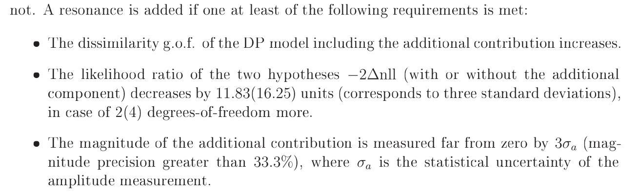
- The point-to-point dissimilarity test will be employed for this purpose:
- Educate the final model by adding new resonances and define the nominal model.
Conclusion
Outlook
Thank you!
AmAn of the \(B_{s}^{0}\rightarrow K_{S}^{0} \pi^{+}\pi^{-}\) decay
Sebastian Ordoñez-Soto
April 14th, 2025
Back up
Sebastian Ordoñez-Soto
AmAn of the \(B_{s}^{0}\rightarrow K_{S}^{0} \pi^{+}\pi^{-}\) decay


Using Truth match MC for signal
\(K_{S}^{0}\pi^{+}\pi^{-}\) Invariant Mass fit
April 14th, 2025
Homemade mass fit
Sebastian Ordoñez-Soto
AmAn of the \(B_{s}^{0}\rightarrow K_{S}^{0} \pi^{+}\pi^{-}\) decay


March 24th, 2025
Homemade mass fit
Sebastian Ordoñez-Soto
AmAn of the \(B_{s}^{0}\rightarrow K_{S}^{0} \pi^{+}\pi^{-}\) decay

March 24th, 2025
Homemade mass fit
Sebastian Ordoñez-Soto
AmAn of the \(B_{s}^{0}\rightarrow K_{S}^{0} \pi^{+}\pi^{-}\) decay


March 24th, 2025
Homemade mass fit
Sebastian Ordoñez-Soto
AmAn of the \(B_{s}^{0}\rightarrow K_{S}^{0} \pi^{+}\pi^{-}\) decay
Current results from the BF analysis:
Results with the homemade fit:
March 24th, 2025
Homemade mass fit
Sebastian Ordoñez-Soto
AmAn of the \(B_{s}^{0}\rightarrow K_{S}^{0} \pi^{+}\pi^{-}\) decay
March 24th, 2025
Using No Truth Match MC for signal
Homemade mass fit
Sebastian Ordoñez-Soto
AmAn of the \(B_{s}^{0}\rightarrow K_{S}^{0} \pi^{+}\pi^{-}\) decay
March 24th, 2025
Using No Truth Match MC for signal
Homemade mass fit
Sebastian Ordoñez-Soto
AmAn of the \(B_{s}^{0}\rightarrow K_{S}^{0} \pi^{+}\pi^{-}\) decay
March 24th, 2025
Using No Truth Match MC for signal


Homemade mass fit
Sebastian Ordoñez-Soto
AmAn of the \(B_{s}^{0}\rightarrow K_{S}^{0} \pi^{+}\pi^{-}\) decay
March 24th, 2025
Using No Truth Match MC for signal


Sebastian Ordoñez-Soto
AmAn of the \(B_{s}^{0}\rightarrow K_{S}^{0} \pi^{+}\pi^{-}\) decay
Efficiency across DP
2018-DD
2018-LL
April 14th, 2025
Sebastian Ordoñez-Soto
AmAn of the \(B_{s}^{0}\rightarrow K_{S}^{0} \pi^{+}\pi^{-}\) decay
Efficiency maps from BF analysis
2017-DD
2017-LL
April 14th, 2025
Sebastian Ordoñez-Soto
AmAn of the \(B_{s}^{0}\rightarrow K_{S}^{0} \pi^{+}\pi^{-}\) decay
Efficiency maps from BF analysis
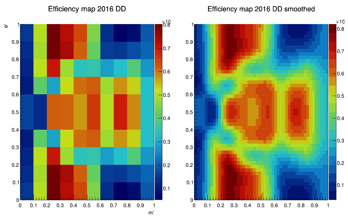
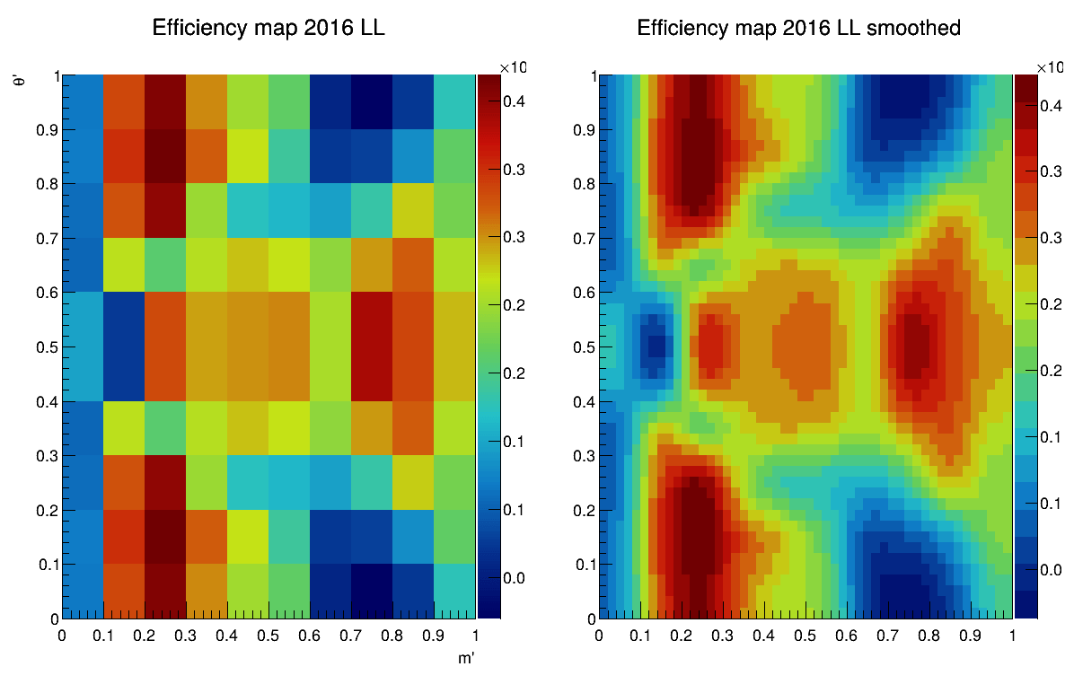
2016-DD
2016-LL
April 14th, 2025
Sebastian Ordoñez-Soto
AmAn of the \(B_{s}^{0}\rightarrow K_{S}^{0} \pi^{+}\pi^{-}\) decay
Efficiency maps from BF analysis
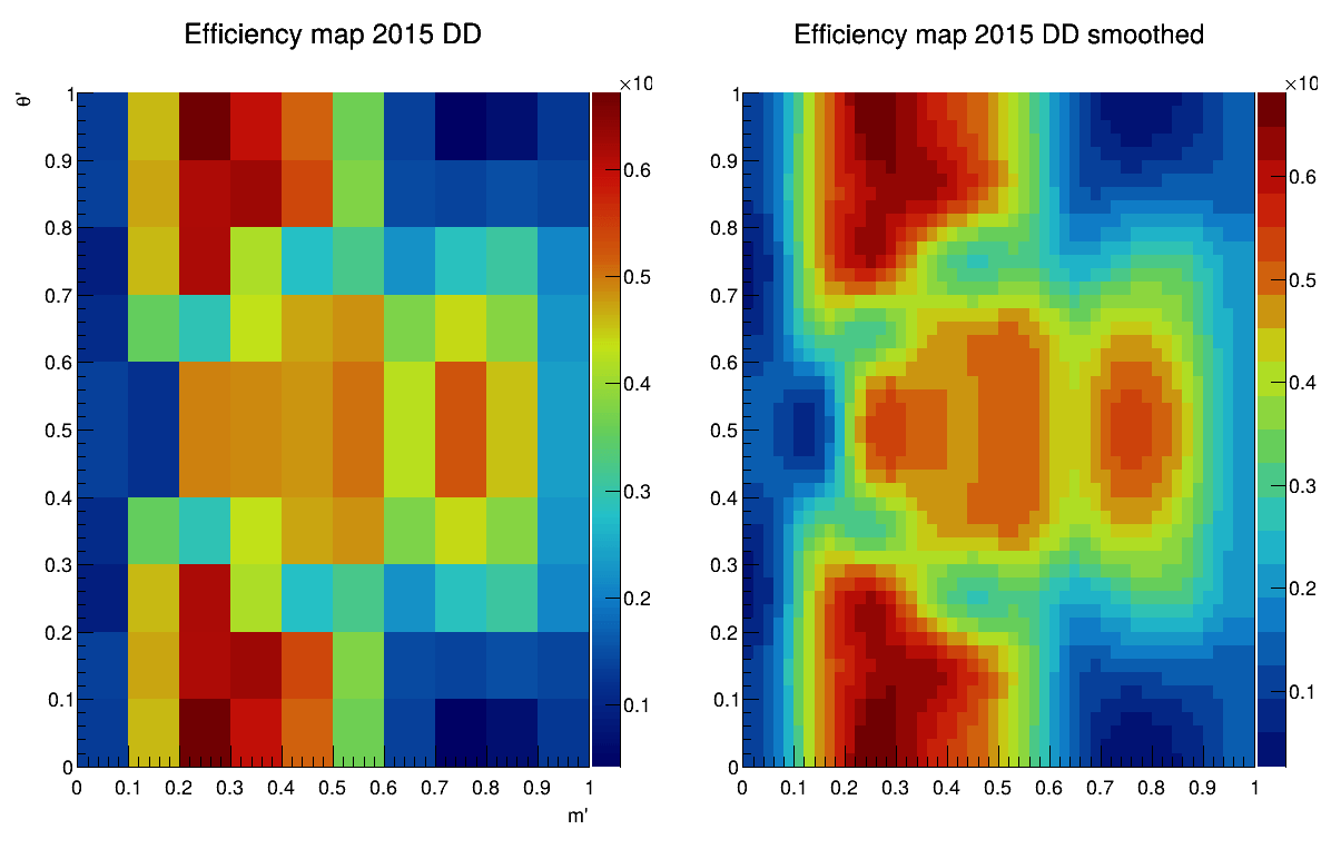
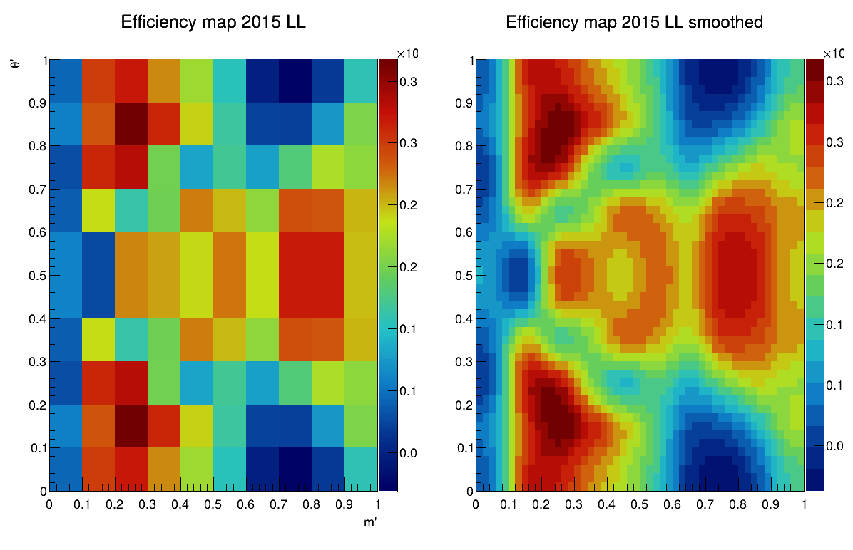
2015-DD
2015-LL
April 14th, 2025
Sebastian Ordoñez-Soto
AmAn of the \(B_{s}^{0}\rightarrow K_{S}^{0} \pi^{+}\pi^{-}\) decay
\(B^{0}_{d}\) background model: Art gallery without asym
April 14th, 2025
Sebastian Ordoñez-Soto
AmAn of the \(B_{s}^{0}\rightarrow K_{S}^{0} \pi^{+}\pi^{-}\) decay
\(B^{0}_{d}\) background model: Art gallery without asym
April 14th, 2025
Sebastian Ordoñez-Soto
AmAn of the \(B_{s}^{0}\rightarrow K_{S}^{0} \pi^{+}\pi^{-}\) decay
\(B^{0}_{d}\) background model: Art gallery without asym
April 14th, 2025
Sebastian Ordoñez-Soto
AmAn of the \(B_{s}^{0}\rightarrow K_{S}^{0} \pi^{+}\pi^{-}\) decay
\(B^{0}_{d}\) background model: Art gallery without asym
April 14th, 2025
Sebastian Ordoñez-Soto
AmAn of the \(B_{s}^{0}\rightarrow K_{S}^{0} \pi^{+}\pi^{-}\) decay
\(B^{0}_{d}\) background model: Art gallery without asym
April 14th, 2025
Sebastian Ordoñez-Soto
AmAn of the \(B_{s}^{0}\rightarrow K_{S}^{0} \pi^{+}\pi^{-}\) decay
\(B^{0}_{d}\) background model: Art gallery without asym
April 14th, 2025
Sebastian Ordoñez-Soto
AmAn of the \(B_{s}^{0}\rightarrow K_{S}^{0} \pi^{+}\pi^{-}\) decay
\(B^{0}_{d}\) background model: Art gallery without asym
April 14th, 2025
Sebastian Ordoñez-Soto
AmAn of the \(B_{s}^{0}\rightarrow K_{S}^{0} \pi^{+}\pi^{-}\) decay
\(B^{0}_{d}\) background model: Art gallery without asym
April 14th, 2025

Sebastian Ordoñez-Soto
AmAn of the \(B_{s}^{0}\rightarrow K_{S}^{0} \pi^{+}\pi^{-}\) decay
\(B^{0}_{d}\) background model: Art gallery without asym
April 14th, 2025

Sebastian Ordoñez-Soto
AmAn of the \(B_{s}^{0}\rightarrow K_{S}^{0} \pi^{+}\pi^{-}\) decay
\(B^{0}_{d}\) background model: Art gallery without asym
April 14th, 2025

Sebastian Ordoñez-Soto
AmAn of the \(B_{s}^{0}\rightarrow K_{S}^{0} \pi^{+}\pi^{-}\) decay
\(B^{0}_{d}\) background model: Art gallery with asym
April 14th, 2025
Sebastian Ordoñez-Soto
AmAn of the \(B_{s}^{0}\rightarrow K_{S}^{0} \pi^{+}\pi^{-}\) decay
\(B^{0}_{d}\) background model: Art gallery

April 14th, 2025
Sebastian Ordoñez-Soto
AmAn of the \(B_{s}^{0}\rightarrow K_{S}^{0} \pi^{+}\pi^{-}\) decay
\(B^{0}_{d}\) background model: Art gallery
April 14th, 2025
Sebastian Ordoñez-Soto
AmAn of the \(B_{s}^{0}\rightarrow K_{S}^{0} \pi^{+}\pi^{-}\) decay
\(B^{0}_{d}\) background model: Art gallery

April 14th, 2025
Sebastian Ordoñez-Soto
AmAn of the \(B_{s}^{0}\rightarrow K_{S}^{0} \pi^{+}\pi^{-}\) decay
\(B^{0}_{d}\) background model: Art gallery


April 14th, 2025
Sebastian Ordoñez-Soto
AmAn of the \(B_{s}^{0}\rightarrow K_{S}^{0} \pi^{+}\pi^{-}\) decay
\(B^{0}_{d}\) background model: Art gallery

April 14th, 2025
Sebastian Ordoñez-Soto
AmAn of the \(B_{s}^{0}\rightarrow K_{S}^{0} \pi^{+}\pi^{-}\) decay
\(B^{0}_{d}\) background model: Art gallery

April 14th, 2025
Sebastian Ordoñez-Soto
AmAn of the \(B_{s}^{0}\rightarrow K_{S}^{0} \pi^{+}\pi^{-}\) decay
\(B^{0}_{d}\) background model: Art gallery

April 14th, 2025
Sebastian Ordoñez-Soto
AmAn of the \(B_{s}^{0}\rightarrow K_{S}^{0} \pi^{+}\pi^{-}\) decay
\(B^{0}_{d}\) background model: Art gallery

April 14th, 2025
Sebastian Ordoñez-Soto
AmAn of the \(B_{s}^{0}\rightarrow K_{S}^{0} \pi^{+}\pi^{-}\) decay
\(B^{0}_{d}\) background model: Art gallery

April 14th, 2025
Sebastian Ordoñez-Soto
AmAn of the \(B_{s}^{0}\rightarrow K_{S}^{0} \pi^{+}\pi^{-}\) decay
Goodness-of-fit test
In short, this is what we do at this stage:
- We do an unbinned maximum likelihood fit of a PDF to the data.
- This fitted PDF is then used to extract the value of some observables from the data.
It is crucial to determine the level of agreement between the fit PDF and the data from a statistical argument (null-hypothesis significance test) \(\Rightarrow\) a goodness-of-fit (g.o.f).
The unbinned Point-to-Point Dissimilarity Method will be used \(\Rightarrow\) event by event
- Notation:
- \(\vec{s} = (s_{-},s_{+}) = (s_{K_{S}\pi^{-}},s_{K_{S}\pi^{+}}) \)
- \(f(\vec{s})\) and \(f_{0}(\vec{s})\): parent/true PDF of the data and test PDF, respectively.
- \(T\): test statistic (TS) \(\Rightarrow\) Larger values correspond to a worse level of agreement.
- \(H_{0}\): Null hypothesis \(\Rightarrow\) "The two samples are drawn from the same PDF".
- \(p\): \(p\)-value \(\Rightarrow\) Significance of any discrepancy between the data and the test PDF
p = \int_T^{\infty} g_{f_0}(T')\, dT' = P(T_{perm} \ge T | H_{0})
How good are your fits? Unbinned multivariate goodness-of-fit tests in high energy physics: http://arxiv.org/abs/1006.3019
April 2nd, 2025
Sebastian Ordoñez-Soto
AmAn of the \(B_{s}^{0}\rightarrow K_{S}^{0} \pi^{+}\pi^{-}\) decay
Goodness-of-fit test
February 19th, 2025
In short, this is what we do at this stage:
- We do an unbinned maximum likelihood fit of a PDF to the data.
- This fitted PDF is then used to extract the value of some observables from the data.
It is crucial to determine the level of agreement between the fit PDF and the data from a statistical argument (null-hypothesis significance test) \(\Rightarrow\) a goodness-of-fit (g.o.f).
We will use the unbinned Point-to-Point Dissimilarity Method.
- Notation:
- \(\vec{s} = (s_{-},s_{+}) = (s_{K_{S}\pi^{-}},s_{K_{S}\pi^{+}}) \)
- \(f(\vec{s})\) and \(f_{0}(\vec{s})\): parent PDF of the data and test PDF, respectively.
- \(T\): test statistic (TS) \(\Rightarrow\) Larger values correspond to a worse level of agreement.
- \(p\): \(p\)-value \(\Rightarrow\) Significance of any discrepancy between the data and the test PDF
p = \int_T^{\infty} g_{f_0}(T')\, dT' = P(T_{perm} \ge T | H_{0})
You want to know whether two sets of points in phase space come from the same underlying distribution
The p-value is the probability of getting a test statistic TTT as large or larger than the observed one, under the null hypothesis.
“If the samples really come from the same distribution, how often would I get a dissimilarity as large as the one I observed, just due to chance?”
Sebastian Ordoñez-Soto
AmAn of the \(B_{s}^{0}\rightarrow K_{S}^{0} \pi^{+}\pi^{-}\) decay
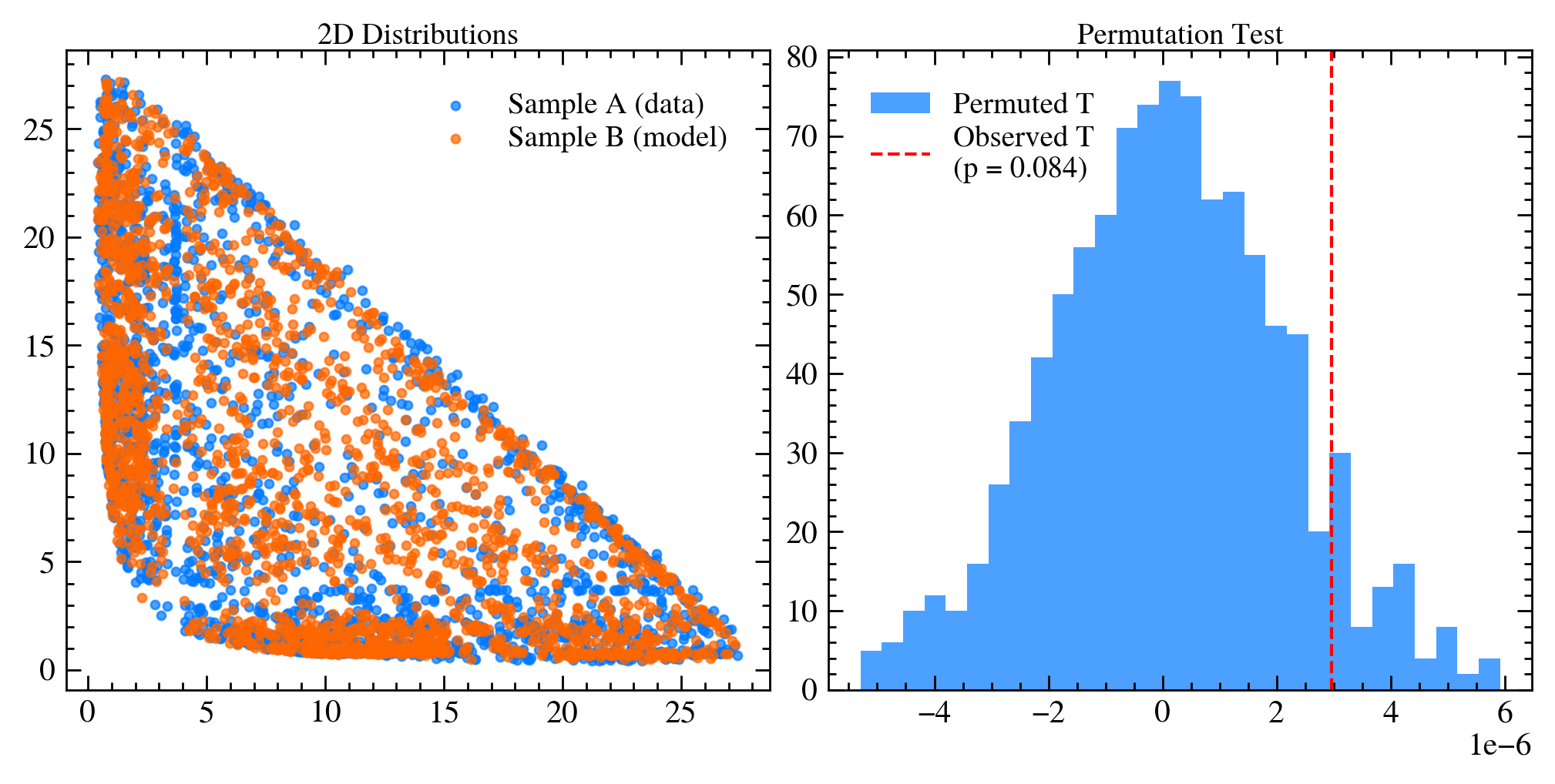
Point-to-Point Dissimilarity Method
Ideally, the difference between \(f\) and \(f_{0}\) could be estimated from the T statistic:
T = \frac{1}{2} \int \left( f(\vec{s}) - f_0(\vec{s}) \right)^2 \, d\vec{s}
It is plausible to postulate a weighting function (WF) \(\psi(|\vec{s}-\vec{s}'|)\) which correlates the difference between the PDF's at different points, such that:
T = \frac{1}{2} \int \int \left( f(\vec{s}) - f_0(\vec{s}) \right) \left( f(\vec{s}') - f_0(\vec{s}') \right) \psi(|\vec{s} - \vec{s}'|) \, d\vec{s} \, d\vec{s}'.
T = \frac{1}{2} \int \int \left[ f(\vec{s}) f(\vec{s}') + f_0(\vec{s}) f_0(\vec{s}') - 2 f(\vec{s}) f_0(\vec{s}') \right] \psi(|\vec{s} - \vec{s}'|) \, d\vec{s} \, d\vec{s}'.
T = \frac{1}{n_d(n_d - 1)} \sum_{\substack{i,j>i}}^{n_d} \psi(|\vec{s}_i^d - \vec{s}_j^d|)
+ \frac{1}{n_{\mathrm{mc}}(n_{\mathrm{mc}} - 1)} \sum_{\substack{i,j>i}}^{n_{\mathrm{mc}}} \psi(|\vec{s}_i^{\mathrm{mc}} - \vec{s}_j^{\mathrm{mc}}|)
- \frac{1}{n_d n_{\mathrm{mc}}} \sum_{i,j}^{n_d, n_{\mathrm{mc}}} \psi(|\vec{s}_i^d - \vec{s}_j^{\mathrm{mc}}|).
This can be approximated by:
The average kernel value between pairs of points if both are drawn from distribution fff
\psi_{\text{exp}}(|\vec{s}_i - \vec{s}_j|) = e^{-|\vec{s}_i - \vec{s}_j|^2 / 2\sigma(\vec{s}_i)\sigma(\vec{s}_j)} \\
\psi_{\text{Log}}(|\vec{s}_{i} - \vec{s}_{j}|) = \ln(|\vec{s}_{i} - \vec{s}_{j}| + \epsilon)
April 2nd, 2025
Sebastian Ordoñez-Soto
AmAn of the \(B_{s}^{0}\rightarrow K_{S}^{0} \pi^{+}\pi^{-}\) decay
Point-to-Point Dissimilarity Method
The distribution of \(T\) for the case \(f = f_{0}\) is not known... How do we estimate a \(p\)-value?
- Permutation sampling
- Combine all data points from both samples into a single pool \(n_{d}+n_{mc}\)
- Randomly reassign points into two new "data" and "MC" samples with sizes \(n_{d}\) and \(n_{mc}\)
- Compute the test statistic \(T_{perm}\) for each permuted pair.
- Repeat this process \(n_{perm}\) times to obtain \(\{T_{perm}^{1},...,T_{perm}^{n_{perm}}\}\)
- The \(p\)-value is the fraction of permutations where \(T_{perm} \geq T \)
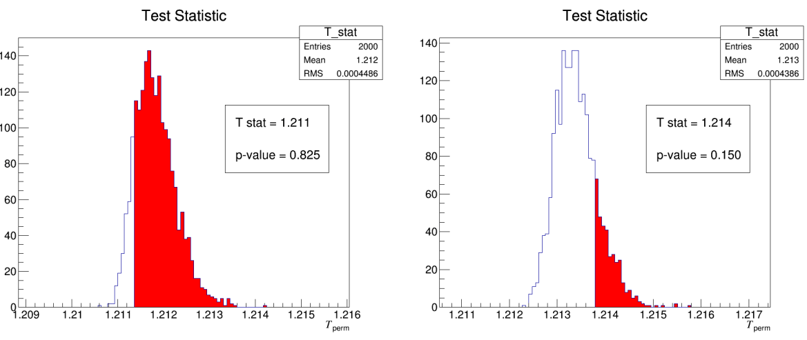
- If \(p\)-value is small:
- The observed dissimilarity is unlikely under \(H_{0}\).
- If \(p\)-value is large:
- The observed dissimilarity could happen by chance.
April 2nd, 2025
Sebastian Ordoñez-Soto
AmAn of the \(B_{s}^{0}\rightarrow K_{S}^{0} \pi^{+}\pi^{-}\) decay
Point-to-Point Dissimilarity Method
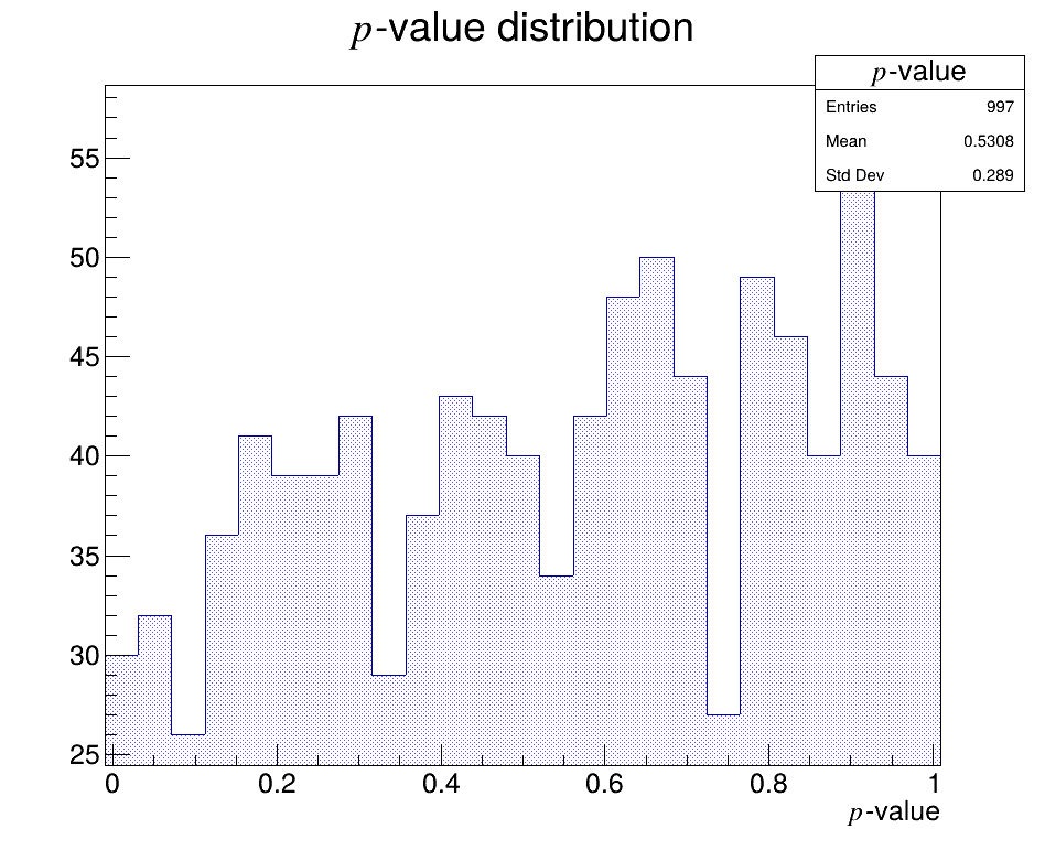
- First test of the method using the Run 1 B2KSpipi PDF
- ~1000 toys
- \(n_{d}=n_{mc} = 100\) (low statistics)
- \(n_{perm}\) = 100
- The logarithmic function is chosen as \(\psi\)
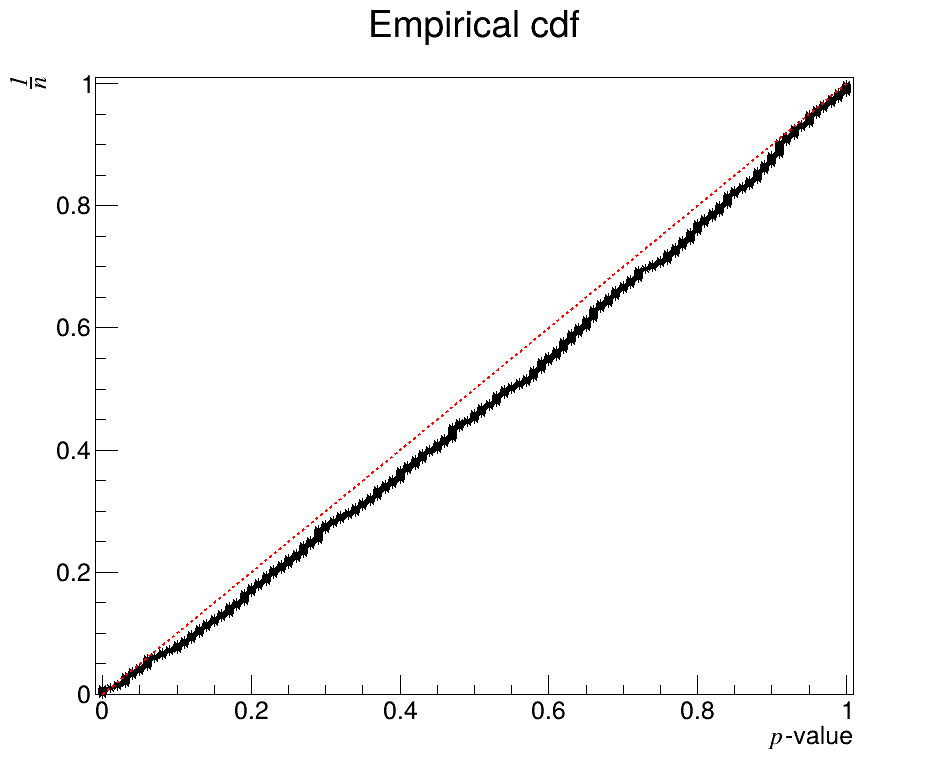
The \(p\)-value is a function of the data and MC, and is therefore itself a random variable
April 2nd, 2025
Sebastian Ordoñez-Soto
AmAn of the \(B_{s}^{0}\rightarrow K_{S}^{0} \pi^{+}\pi^{-}\) decay
Towards the nominal DP model
Run 1 procedure for B2KSpipi
April 2nd, 2025
Sebastian Ordoñez-Soto
AmAn of the \(B_{s}^{0}\rightarrow K_{S}^{0} \pi^{+}\pi^{-}\) decay
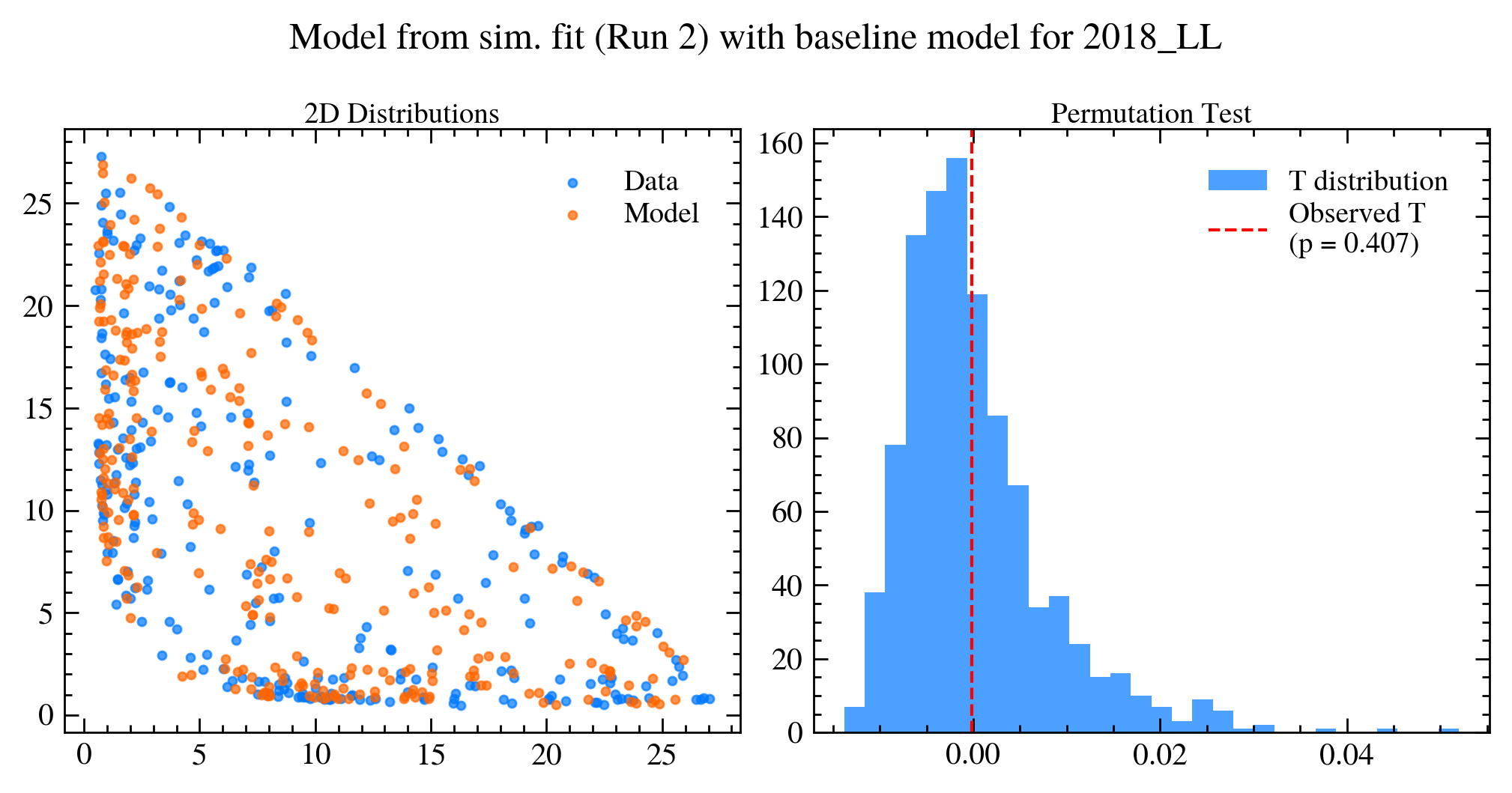
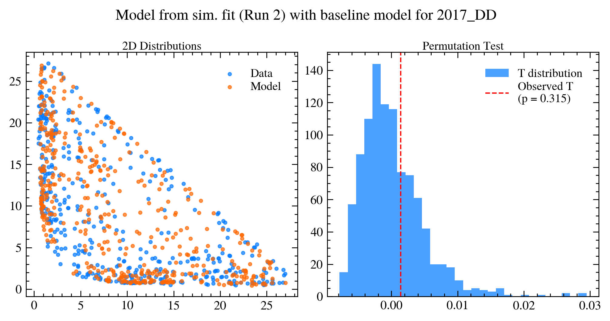
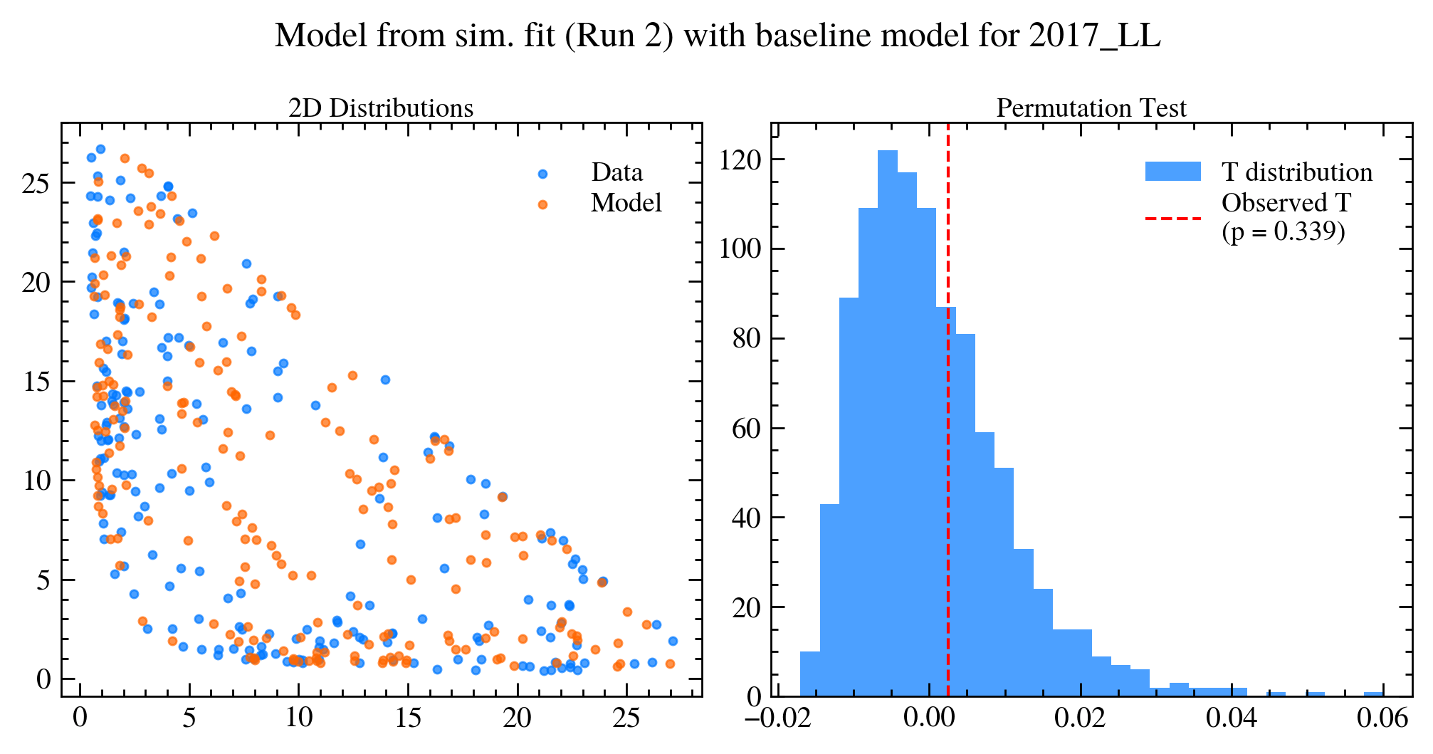
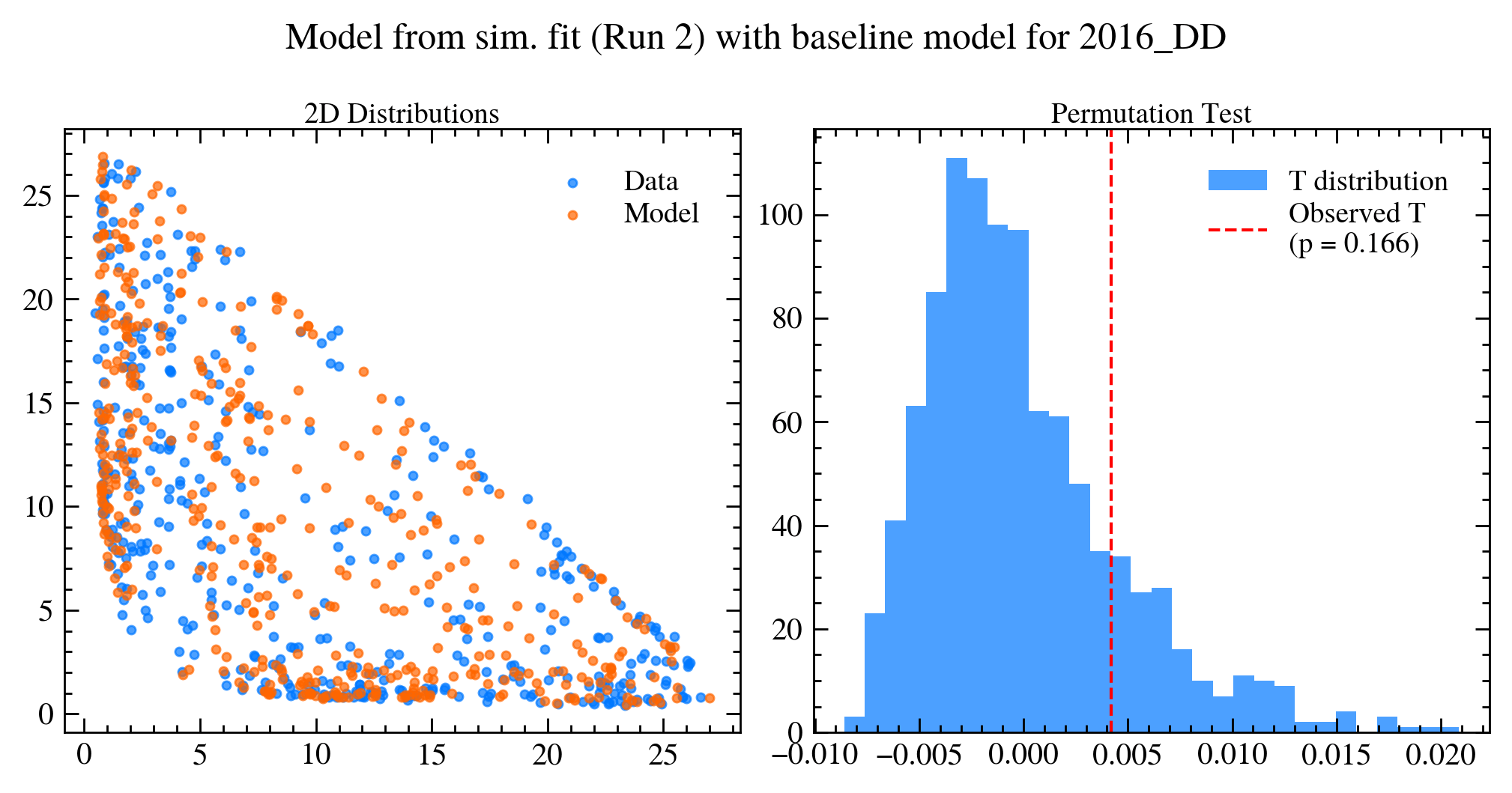
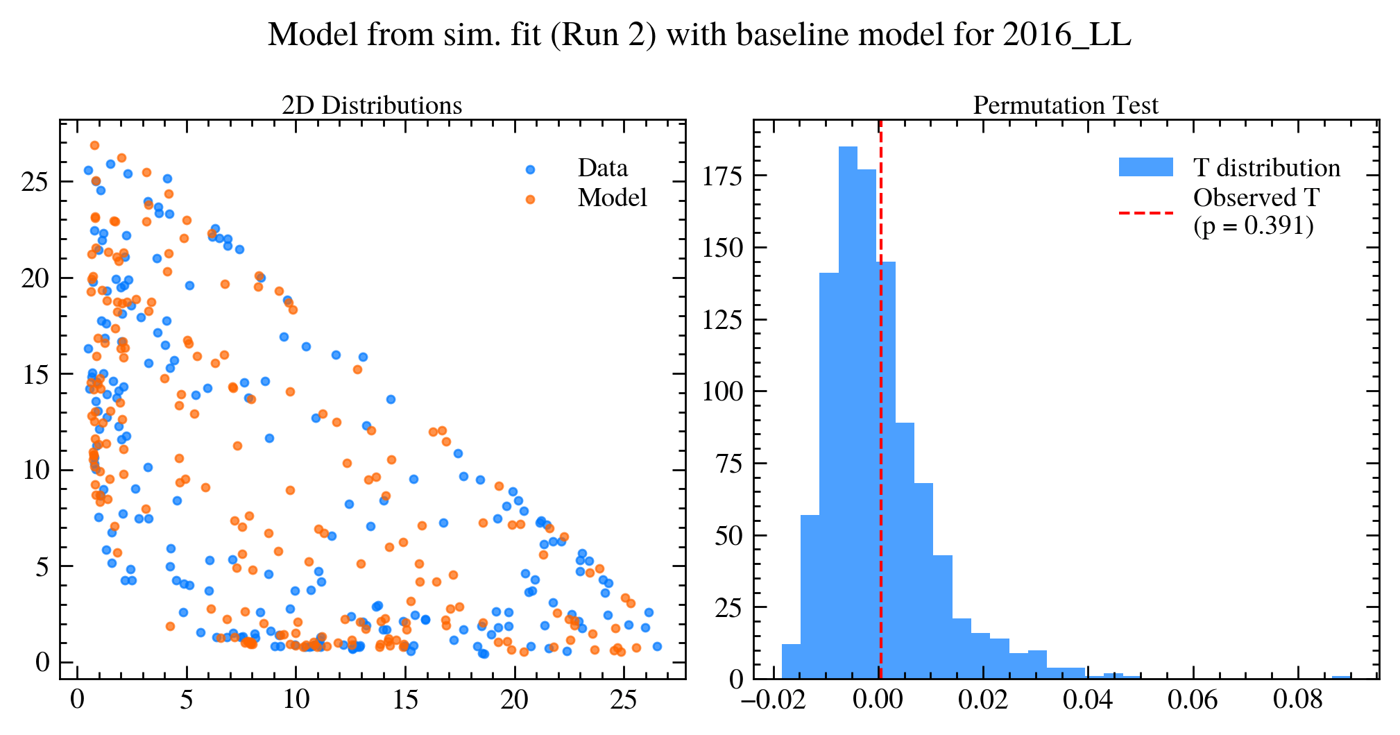
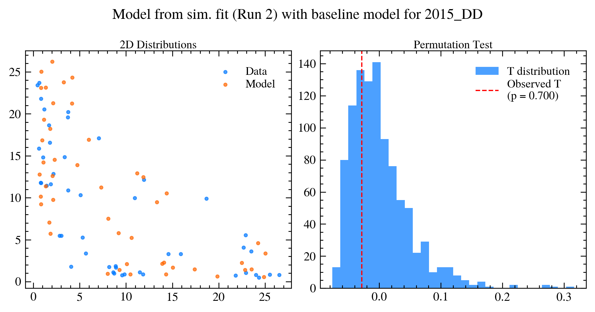
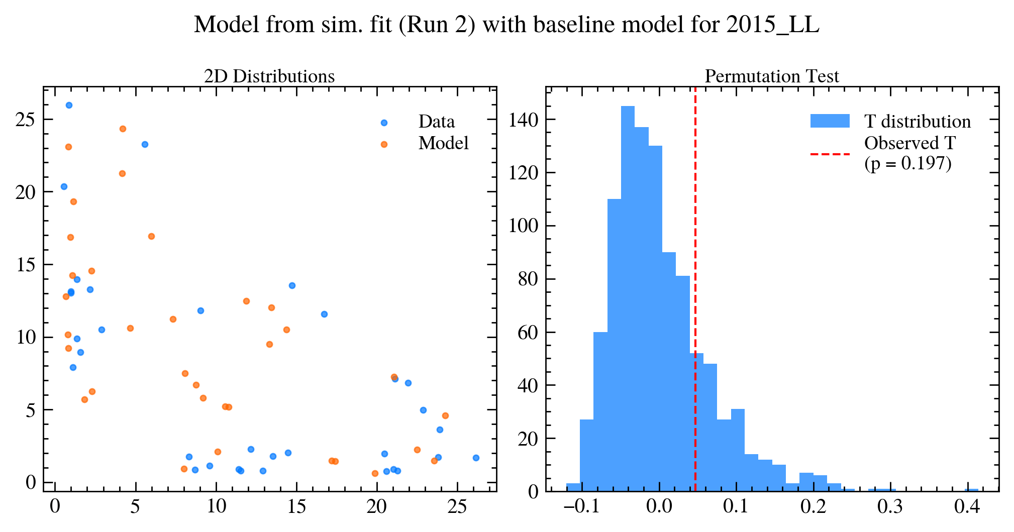
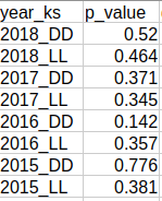
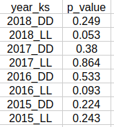
Dissimilarity test results
Baseline model
May 2025
\boxed{p_{\text{global}} = 0.38}
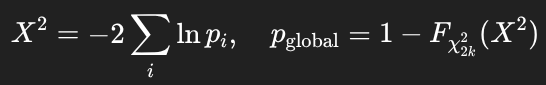
Fisher's method
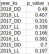
P-values per sub-sample baseline
Global p-value (Fisher) baseline: 0.38
Global p-value (Stouffer) baseline: 0.16
Sebastian Ordoñez-Soto
AmAn of the \(B_{s}^{0}\rightarrow K_{S}^{0} \pi^{+}\pi^{-}\) decay
Dissimilarity test results
Baseline model
May 2025
Sebastian Ordoñez-Soto
AmAn of the \(B_{s}^{0}\rightarrow K_{S}^{0} \pi^{+}\pi^{-}\) decay
Dissimilarity test results
Baseline model
May 2025
Sebastian Ordoñez-Soto
AmAn of the \(B_{s}^{0}\rightarrow K_{S}^{0} \pi^{+}\pi^{-}\) decay
Dissimilarity test results
Baseline model
May 2025
Sebastian Ordoñez-Soto
AmAn of the \(B_{s}^{0}\rightarrow K_{S}^{0} \pi^{+}\pi^{-}\) decay
Dissimilarity test results
Baseline model
May 2025
Sebastian Ordoñez-Soto
AmAn of the \(B_{s}^{0}\rightarrow K_{S}^{0} \pi^{+}\pi^{-}\) decay
Dissimilarity test results
Baseline model
May 2025
Sebastian Ordoñez-Soto
AmAn of the \(B_{s}^{0}\rightarrow K_{S}^{0} \pi^{+}\pi^{-}\) decay
Dissimilarity test results
Baseline model
May 2025
Sebastian Ordoñez-Soto
AmAn of the \(B_{s}^{0}\rightarrow K_{S}^{0} \pi^{+}\pi^{-}\) decay
Dissimilarity test results
Baseline model
May 2025
Sebastian Ordoñez-Soto
AmAn of the \(B_{s}^{0}\rightarrow K_{S}^{0} \pi^{+}\pi^{-}\) decay
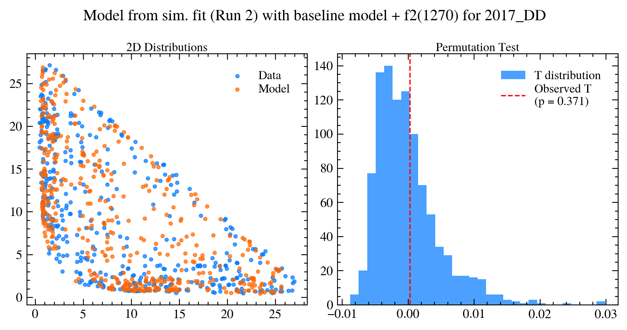
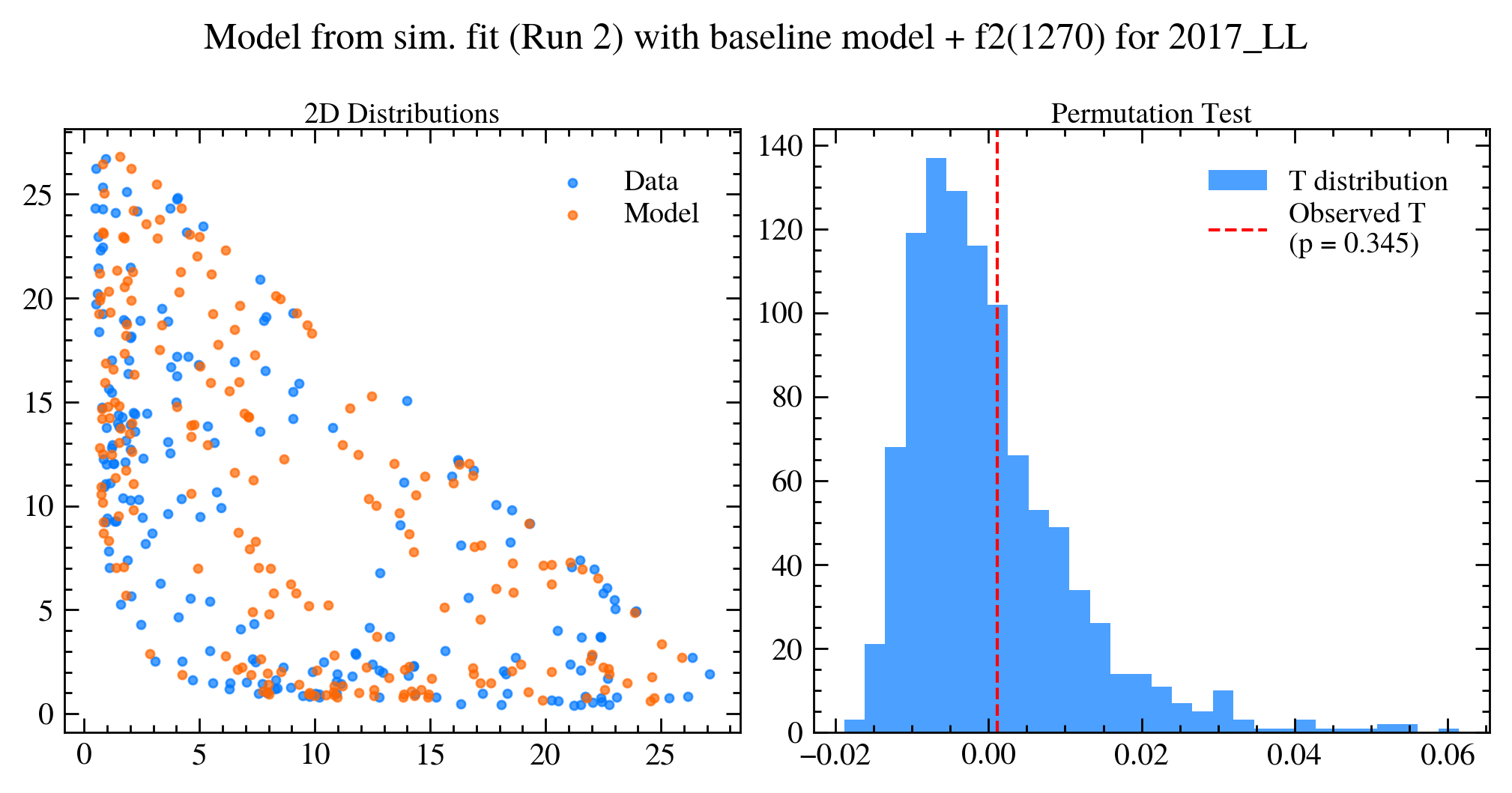
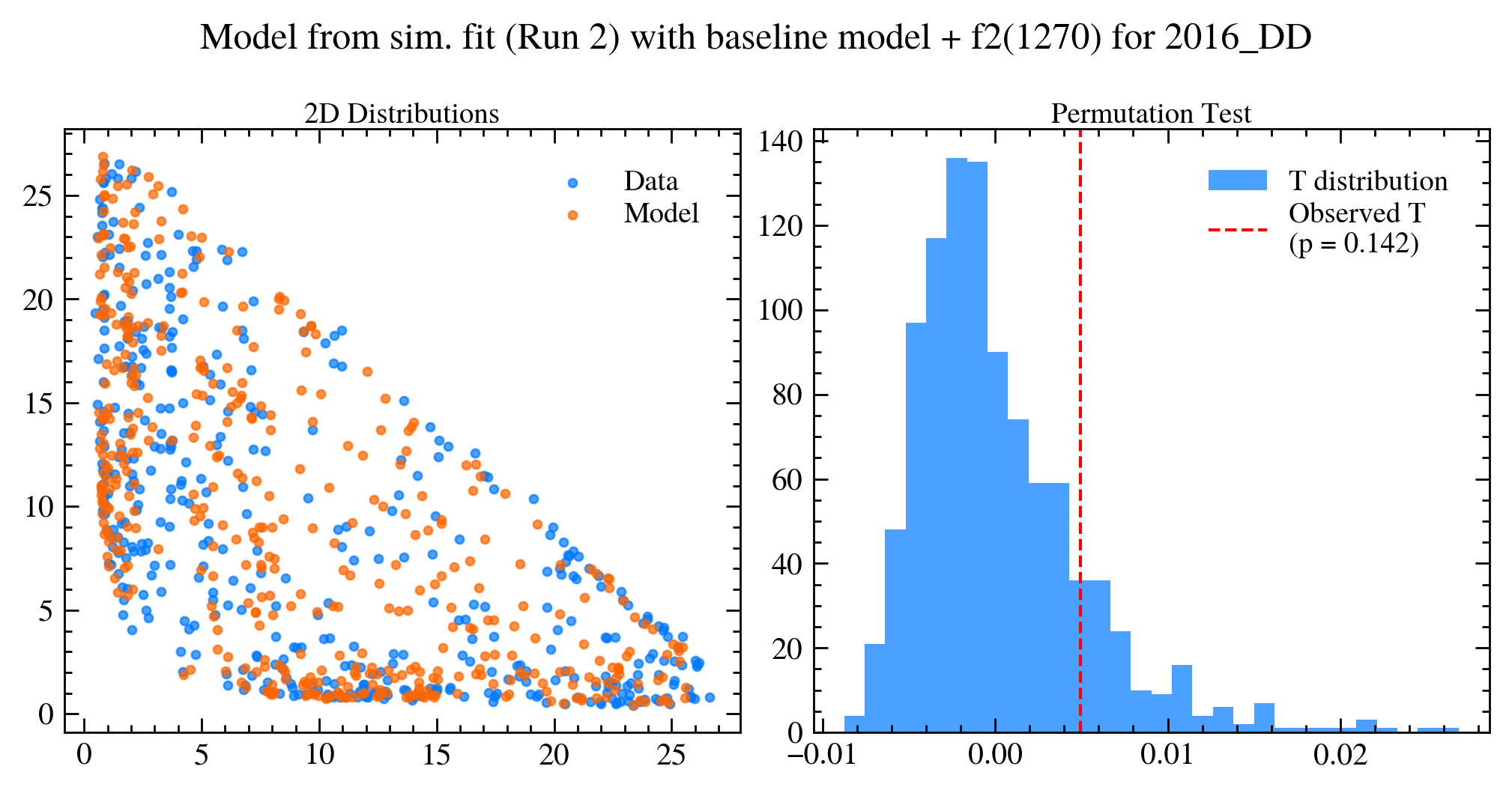
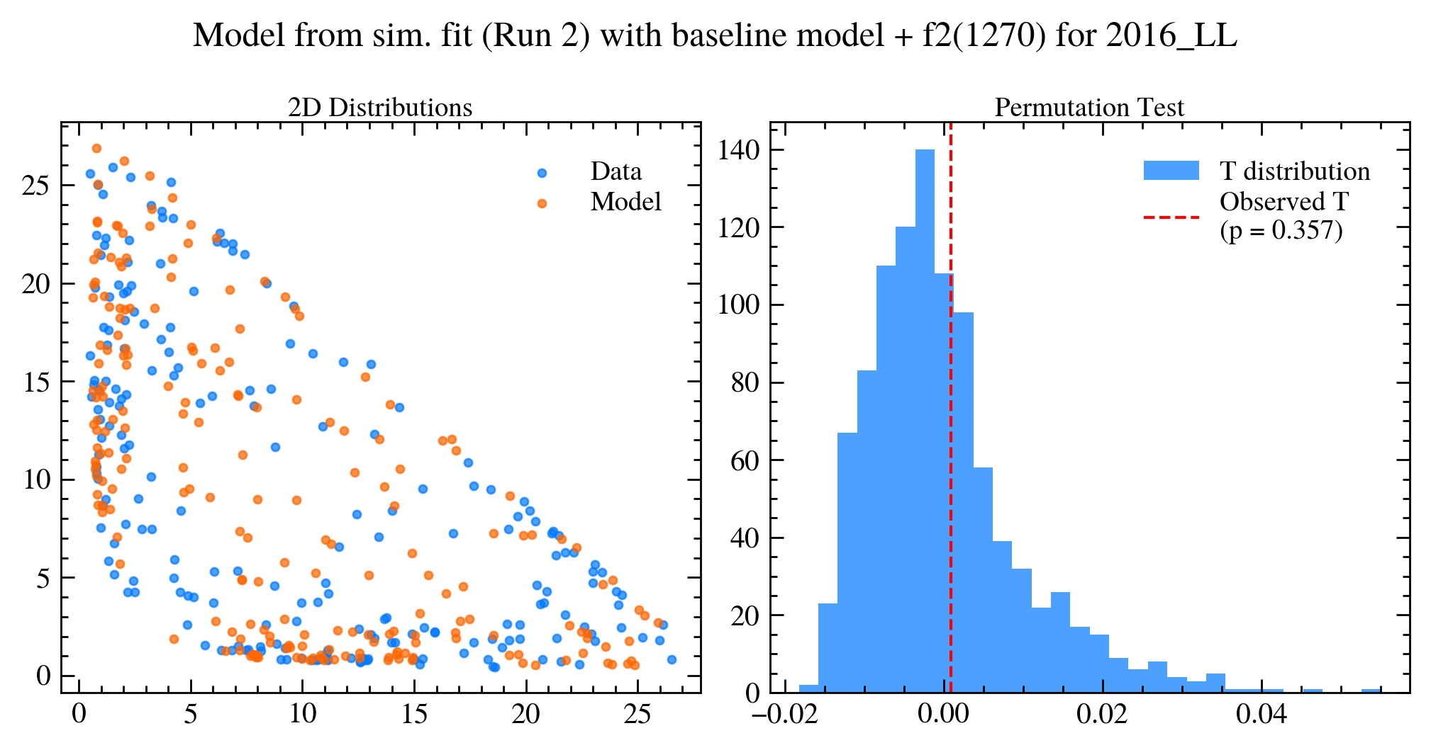
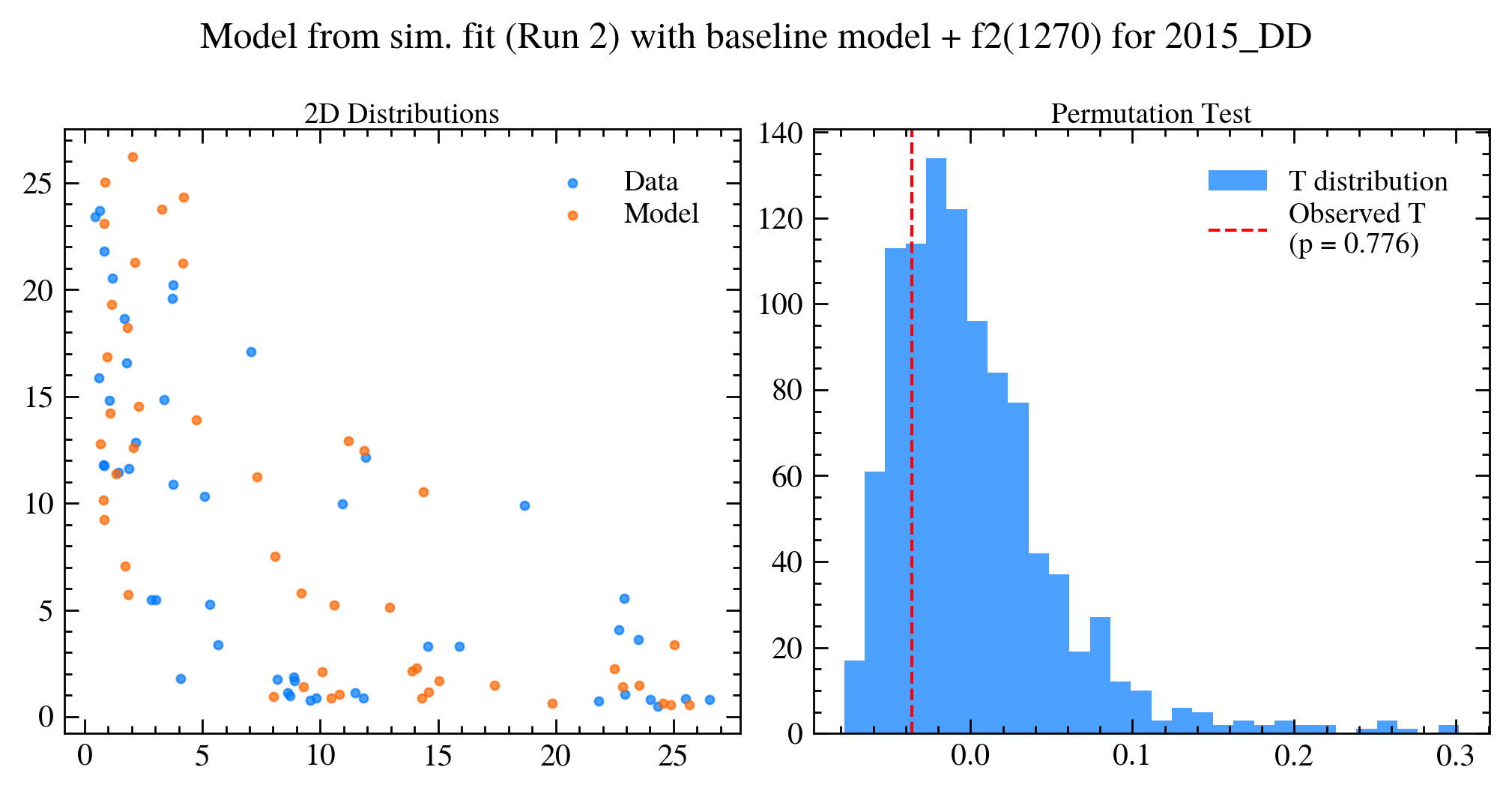
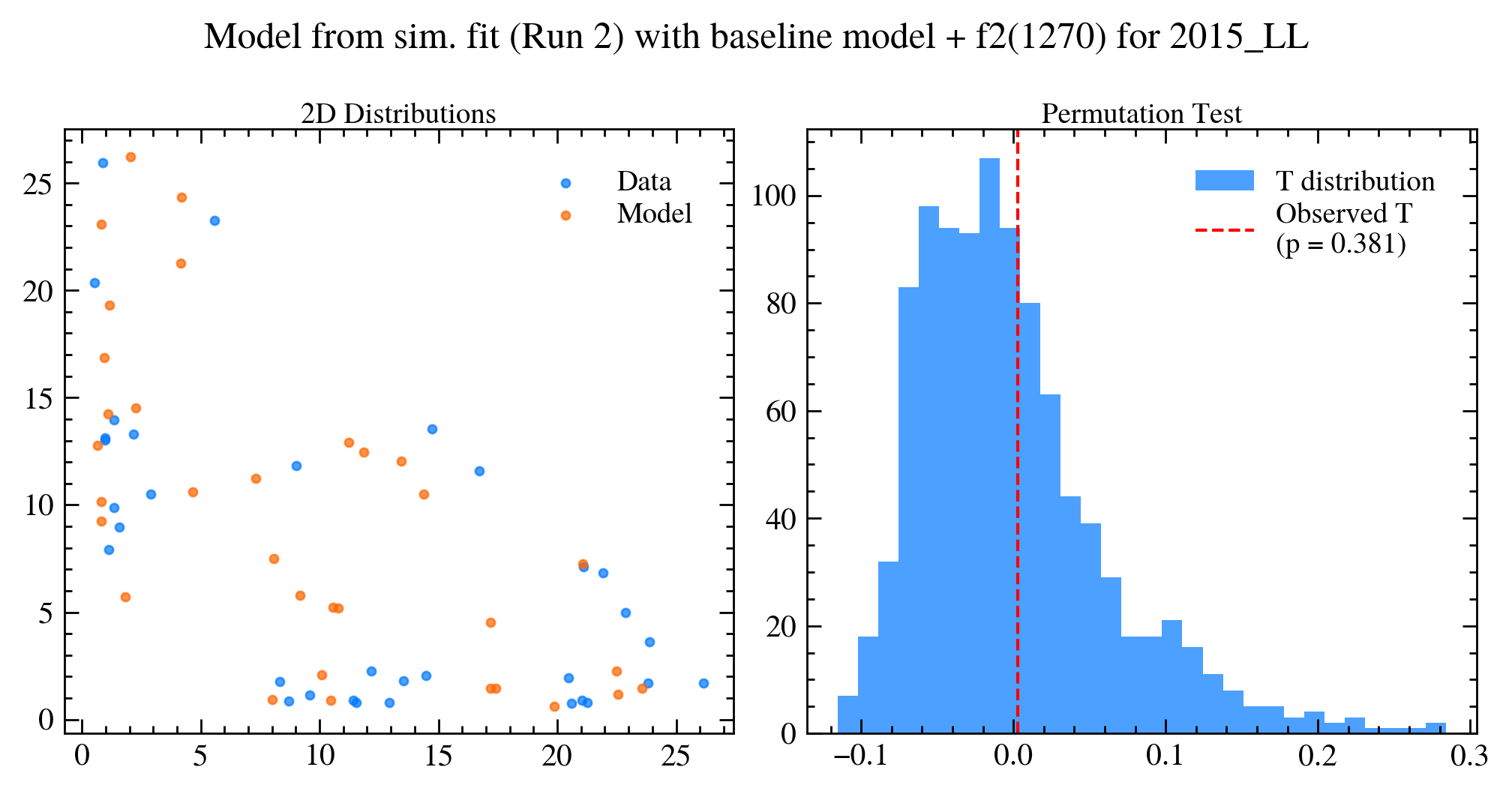
Dissimilarity test results
Baseline model+f2
May 2025
\boxed{p_{\text{global}} = 0.5}
Fisher's method
P-values per sub-sample baseline+f2
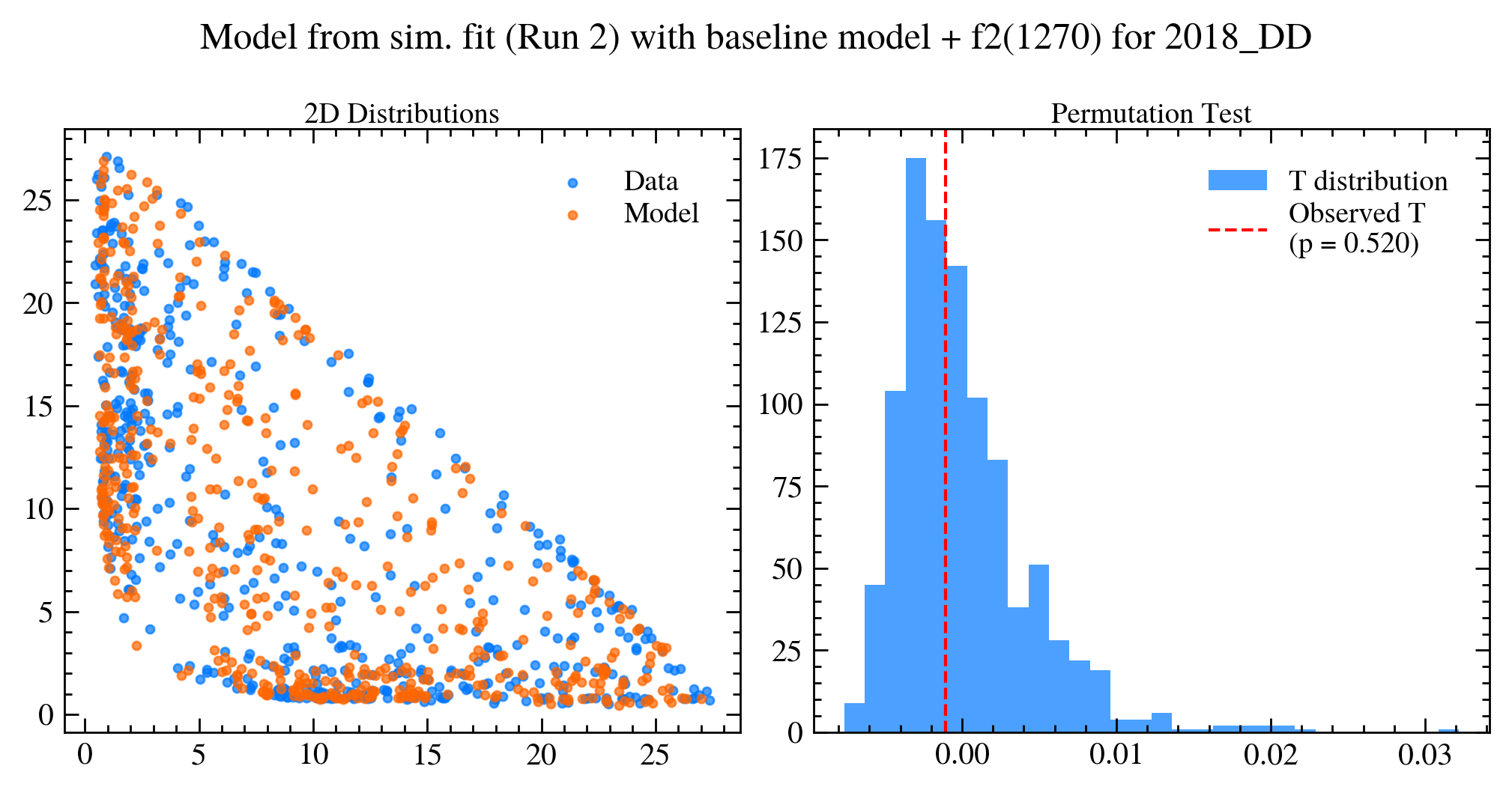
Global p-value (Fisher) baseline+f2: 0.5
Global p-value (Stouffer) baseline+f2: 0.21
P-values per sub-sample
baseline
Sebastian Ordoñez-Soto
AmAn of the \(B_{s}^{0}\rightarrow K_{S}^{0} \pi^{+}\pi^{-}\) decay
Dissimilarity test results
Baseline model+f2
May 2025
Sebastian Ordoñez-Soto
AmAn of the \(B_{s}^{0}\rightarrow K_{S}^{0} \pi^{+}\pi^{-}\) decay
Dissimilarity test results
Baseline model+f2
May 2025
Sebastian Ordoñez-Soto
AmAn of the \(B_{s}^{0}\rightarrow K_{S}^{0} \pi^{+}\pi^{-}\) decay
Dissimilarity test results
Baseline model+f2
May 2025
Sebastian Ordoñez-Soto
AmAn of the \(B_{s}^{0}\rightarrow K_{S}^{0} \pi^{+}\pi^{-}\) decay
Dissimilarity test results
Baseline model+f2
May 2025
Sebastian Ordoñez-Soto
AmAn of the \(B_{s}^{0}\rightarrow K_{S}^{0} \pi^{+}\pi^{-}\) decay
Dissimilarity test results
Baseline model+f2
May 2025
Sebastian Ordoñez-Soto
AmAn of the \(B_{s}^{0}\rightarrow K_{S}^{0} \pi^{+}\pi^{-}\) decay
Dissimilarity test results
Baseline model+f2
May 2025
Sebastian Ordoñez-Soto
AmAn of the \(B_{s}^{0}\rightarrow K_{S}^{0} \pi^{+}\pi^{-}\) decay
Dissimilarity test results
Baseline model+f2
May 2025
Sebastian Ordoñez-Soto
AmAn of the \(B_{s}^{0}\rightarrow K_{S}^{0} \pi^{+}\pi^{-}\) decay
Dissimilarity test results
May 2025
p-values per sub-sample baseline+f2
Global p-value (Fisher) baseline+f2: 0.12
Global p-value (Stouffer) baseline+f2: 0.1
P-values per sub-sample
baseline
Comparison using gaussian correlation function
Global p-value (Fisher) baseline: 0.12
Global p-value (Stouffer) baseline: 0.11

p-value full Run 2
baseline+f2
Sebastian Ordoñez-Soto
AmAn of the \(B_{s}^{0}\rightarrow K_{S}^{0} \pi^{+}\pi^{-}\) decay
Combinatorial background model
Run 2 DD merged
February 17th, 2025
Sebastian Ordoñez-Soto
AmAn of the \(B_{s}^{0}\rightarrow K_{S}^{0} \pi^{+}\pi^{-}\) decay
Combinatorial background model
February 3rd, 2025
2018 DD
Sebastian Ordoñez-Soto
AmAn of the \(B_{s}^{0}\rightarrow K_{S}^{0} \pi^{+}\pi^{-}\) decay
Combinatorial background model
February 3rd, 2025
2017 DD
Sebastian Ordoñez-Soto
AmAn of the \(B_{s}^{0}\rightarrow K_{S}^{0} \pi^{+}\pi^{-}\) decay
Combinatorial background model
February 3rd, 2025
2016 DD
Sebastian Ordoñez-Soto
AmAn of the \(B_{s}^{0}\rightarrow K_{S}^{0} \pi^{+}\pi^{-}\) decay
Combinatorial background model
February 3rd, 2025
2015 DD
Sebastian Ordoñez-Soto
AmAn of the \(B_{s}^{0}\rightarrow K_{S}^{0} \pi^{+}\pi^{-}\) decay
Combinatorial background model
Run 2 LL merged
February 17th, 2025
Sebastian Ordoñez-Soto
AmAn of the \(B_{s}^{0}\rightarrow K_{S}^{0} \pi^{+}\pi^{-}\) decay
Combinatorial background model
February 3rd, 2025
2018 LL
Sebastian Ordoñez-Soto
AmAn of the \(B_{s}^{0}\rightarrow K_{S}^{0} \pi^{+}\pi^{-}\) decay
Combinatorial background model
February 3rd, 2025
2017 LL
Sebastian Ordoñez-Soto
AmAn of the \(B_{s}^{0}\rightarrow K_{S}^{0} \pi^{+}\pi^{-}\) decay
Combinatorial background model
February 3rd, 2025
2016 LL
Sebastian Ordoñez-Soto
AmAn of the \(B_{s}^{0}\rightarrow K_{S}^{0} \pi^{+}\pi^{-}\) decay
Combinatorial background model
February 3rd, 2025
2015 LL
Sebastian Ordoñez-Soto
AmAn of the \(B_{s}^{0}\rightarrow K_{S}^{0} \pi^{+}\pi^{-}\) decay
Combinatorial background model
Run 2 DD + LL categories merged
February 19th, 2025
Sebastian Ordoñez-Soto
AmAn of the \(B_{s}^{0}\rightarrow K_{S}^{0} \pi^{+}\pi^{-}\) decay
Combinatorial background model
February 3rd, 2025
2018 DD + LL categories merged
Sebastian Ordoñez-Soto
AmAn of the \(B_{s}^{0}\rightarrow K_{S}^{0} \pi^{+}\pi^{-}\) decay
Combinatorial background model
February 3rd, 2025
2017 DD + LL categories merged
Sebastian Ordoñez-Soto
AmAn of the \(B_{s}^{0}\rightarrow K_{S}^{0} \pi^{+}\pi^{-}\) decay
Combinatorial background model
February 3rd, 2025
2016 DD + LL categories merged
Sebastian Ordoñez-Soto
AmAn of the \(B_{s}^{0}\rightarrow K_{S}^{0} \pi^{+}\pi^{-}\) decay
Combinatorial background model
February 3rd, 2025
2015 DD + LL categories merged
[Bs2KSpipi AmAn/Anatomy+Preliminary results] B2KShh' mu-Group meeting-14/04/25
By Sebastian Ordoñez


