Study of the \(K\bar{K}\) S-wave amplitude near threshold in the \(D^{+}\rightarrow K^{-}K^{+}K^{+}\) decay


Juan Sebastián Ordoñez Soto
Supervised by D. Milanés and C. Sandoval
Master thesis defense
Grupo de Partículas FENYX-UN
Departamento de Física, Universidad Nacional de Colombia
Bogotá, Colombia
January 24th, 2025
- Scientific context
- Experimental Setup
- Amplitude Analysis of the \(D^{+}\rightarrow K^{-}K^{+}K^{+}\) decay
- Summary and conclusion
Outline
-
Sebastian Ordoñez-Soto
January 24th, 2025
Scientific Context
The Standard Model
Scientific context
Sebastian Ordoñez-Soto
January 24th, 2025
-
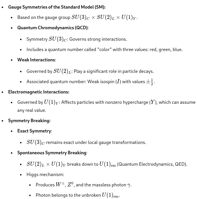
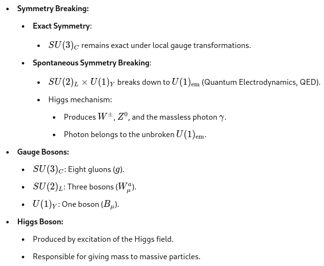
The Standard Model (SM) is the quantum field theory which describes strong and electroweak interactions.
- Based on: local gauge invariance \(\text{SU}(3)_{C}\times \text{SU}(2)_{L} \times \text{U}(1)_{Y}\) and spontaneous symmetry breaking
- Flavour physics relates to the existence of different families of quarks and how they couple to each other.
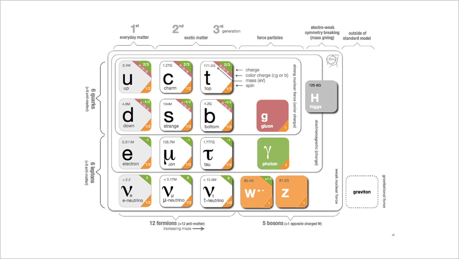
https://cds.cern.ch/record/1473657
The strong sector of the SM is not perturbative at low-energy scales!
Three-body decays of charmed mesons
Scientific context
Sebastian Ordoñez-Soto
January 24th, 2025
-
Lack of description from first principles
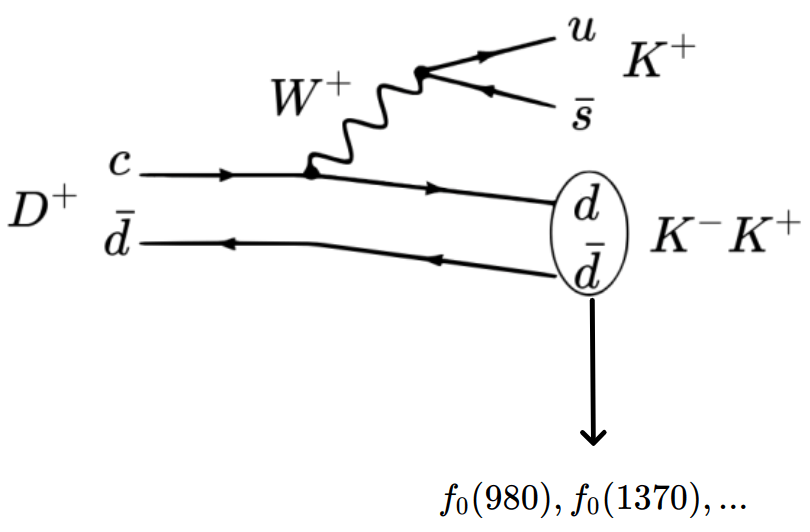
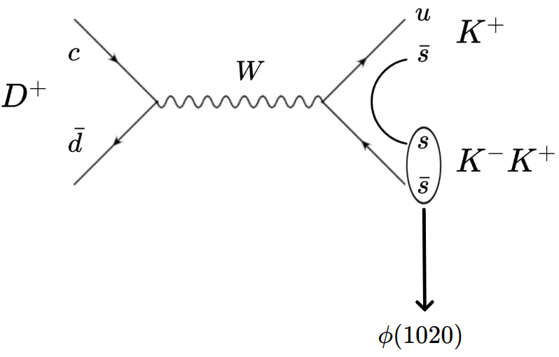
- Weak decay of the charm quark and the formation of the hadrons.
-
The dynamics are assumed to be mainly driven by two-body interactions.
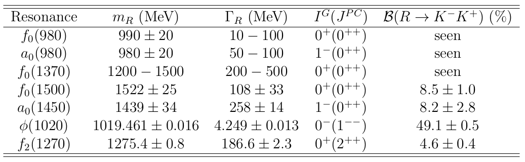
- Rich resonant structure \(\Rightarrow\) Scalars: \(f_{0}(980)\), \(a_{0}(980)\), \(f_{0}(1370)\),... Vectors: \(\phi(1020)\),...
Multi-body decays of \(D\) mesons have been used for light-meson spectroscopy in recent decades.
The \(D^{+}\rightarrow K^{-}K^{+}K^{+}\) decay is an excellent lab for the measurement of the \(K\bar{K}\) amplitude in \(\mathcal{S}\)-wave.
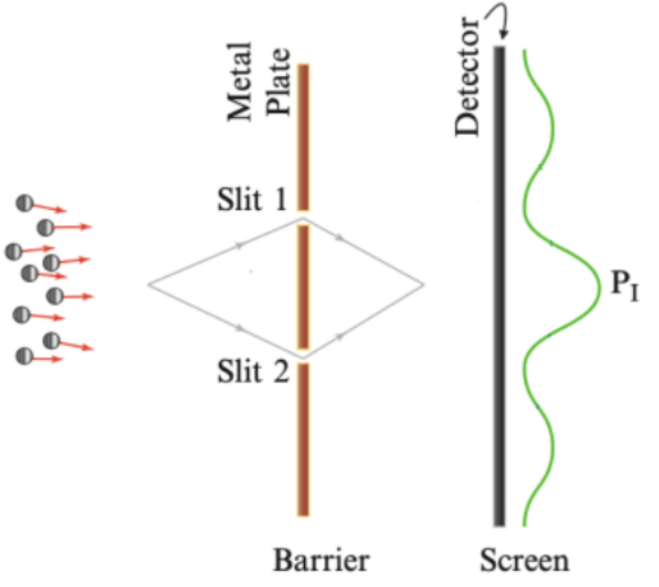
1=|\Psi|^2 = |\Psi_1 + \Psi_2|^2 = |\Psi_1|^2 + |\Psi_2|^2 + 2\mathrm{Re}[\Psi_1 \Psi_2^*]
|\Psi|^2
\Psi_{1}
\Psi_{2}
Amplitude analysis and Dalitz plot
Scientific context
Sebastian Ordoñez-Soto
January 24th, 2025
\boxed{\mathrm{d}\Gamma = \frac{1}{(2\pi)^3} \frac{|\mathcal{M(s_{12},s_{13})}|^2}{32 m_{D^+}} \mathrm{d}s_{12} \mathrm{d}s_{13}
}
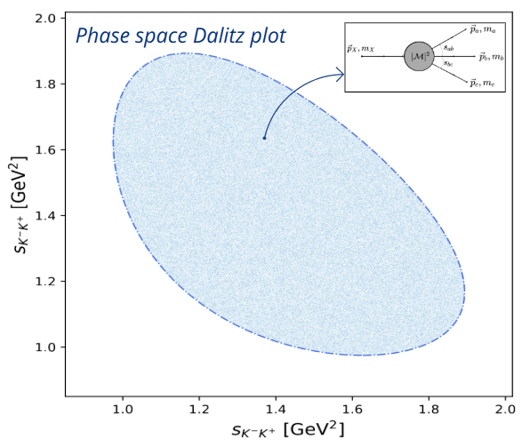
- Dalitz plot (DP) \(\Rightarrow\) Two-dimensional representation of the phase space of three-body decays.
-
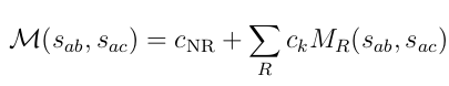
Isobar model (IM) \(\Rightarrow\) Parameterization of the decay amplitude \(\mathcal{M}\).
- Coherent sum of a non-resonant (NR) component and resonant amplitudes.
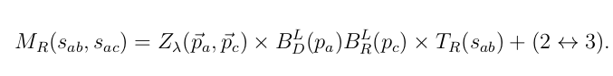
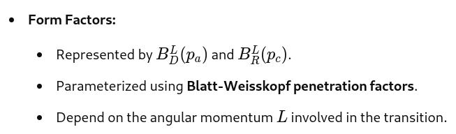
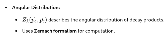
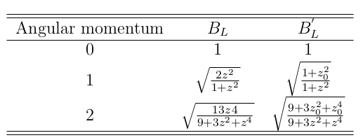
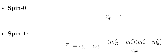
- Each resonance is described by \(\Rightarrow\) \(M_k(s_{12}, s_{13}) = Z_\lambda(\vec{p}_1, \vec{p}_3) \times B_D^L(p_1) B_R^L(p_3) \times T_{k} (s_{12}) + (2\leftrightarrow 3)\)
\boxed{|\mathcal{M}(s_{12}, s_{13}) |^2 = \left| c_{\text{NR}} + \sum_k c_k M_k(s_{12}, s_{13}) \right|^2 }
\boxed{c_k = a_{k} e^{i\delta_{k}}}
Isobar parameters
m^{2}(K_{1}^{-}K_{2}^{+}) = s_{K^{-}K^{+}} = s_{12}\\
m^{2}(K_{1}^{-}K_{3}^{+}) = s_{K^{-}K^{+}} = s_{13}
Notation:
Experimental Setup
The Large Hadron Collider (LHC)
Experimental Setup
Sebastian Ordoñez-Soto
January 24th, 2025
-
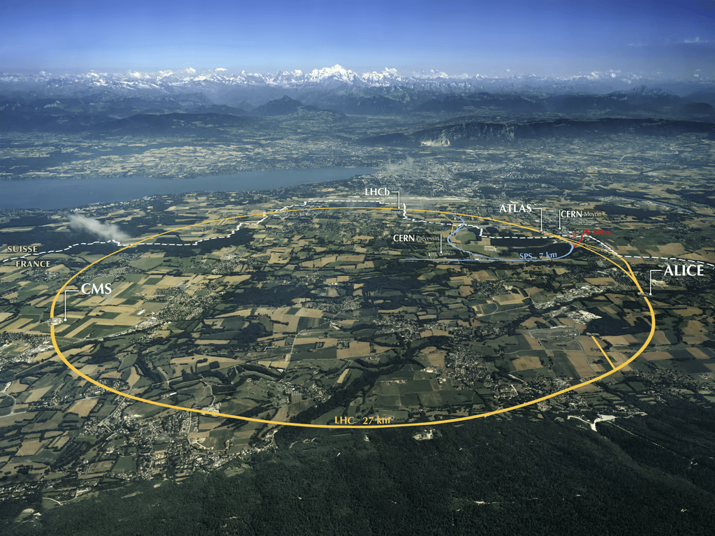
LHC is the world’s largest and most powerful particle accelerator:
- Center-of-mass energy \(\sqrt{s}\)
- Collision rate \(\Rightarrow\) Luminosity \(L=\int\frac{N^{2}f}{4\pi\sigma_{eff}}\text{d}t\)
- It collides protons (\(pp\)) and heavy ions.
-
Main detectors:
- ATLAS, CMS, ALICE and LHCb
-
This thesis uses \(D\rightarrow 3K\) candidates from \(pp\) collisions recorded by LHCb during the Run 2:
- 2016-2018 at \(\sqrt{s}=13\) TeV and \(L=5.6\) fb\(^{-1}\)
- Produced \(c\bar{c}\) pairs: \(N_{c\bar{c}}\approx 8\times10^{15}\)
27 km circumference collider at CERN, near Geneva.
The main objective of the LHC is to explore physics beyond the SM.
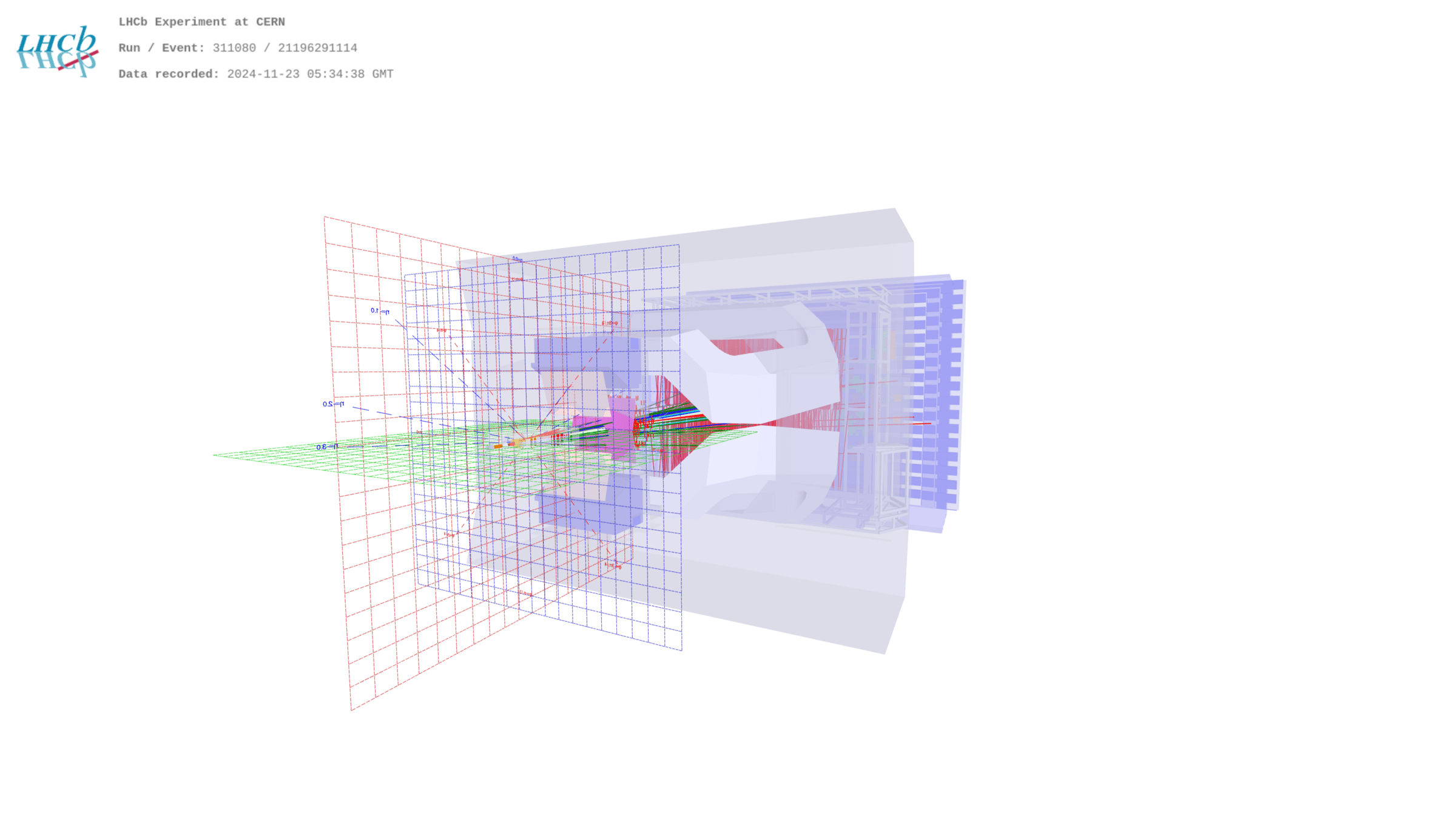
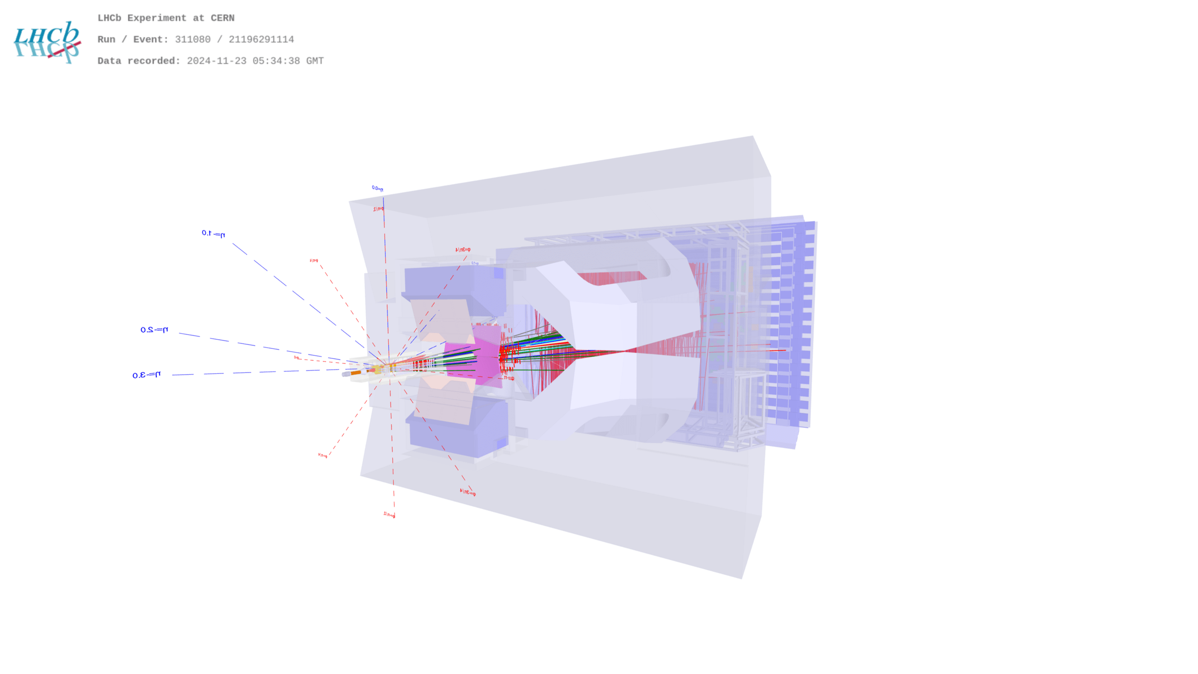
The LHCb detector during Run 2
Experimental Setup
Sebastian Ordoñez-Soto
January 24th, 2025
- LHCb is focused on heavy-flavour (HF) physics studies through \(b\) and \(c\) hadrons decays.
- CP violation searches
- Rare decays
- HF production and spectroscopy
- Main components:
- Tracking system (TS)
- Particle Identification (PID) system
- Trigger system (hardware and software)
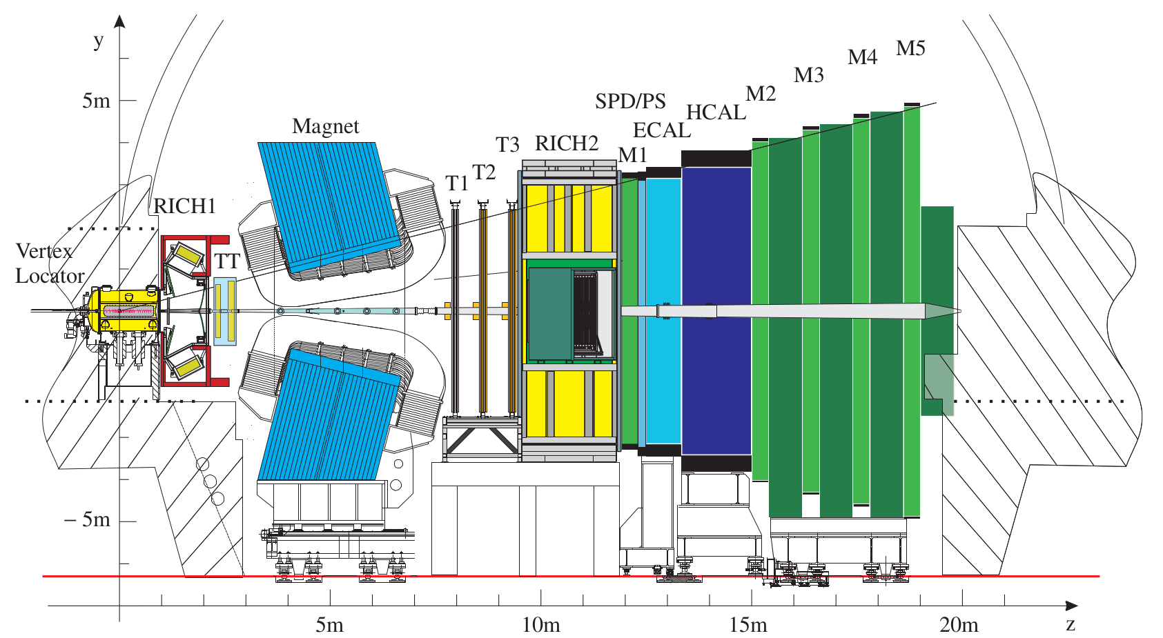
Single-arm forward detector
These components altogether allow to identify and measure –with high precision– the physical properties of particles produced after the \(pp\) collisions
Stable particles in LHCb terminology: \(\pi^{\pm}\), \(K^{\pm}\), \(p\), \(e^{\pm}\), \(\mu^{\pm}\), \(\gamma\).
The tracking and PID systems of LHCb
Experimental Setup
Sebastian Ordoñez-Soto
January 24th, 2025
- TS allows to measure the momenta of charged particles and the position of the primary and decay vertices.
- Vertex Locator \(\rightarrow\) closest to the interaction point
- Dipole magnet \(\rightarrow\) curves trajectories
- Tracker Turicensis (TT)
- Inner and Outer trackers
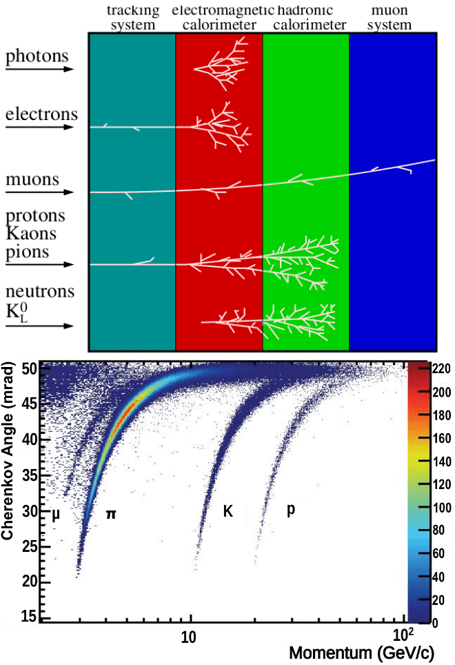
- PID system assign an identity with a given probability to the different tracks.
- The Ring Imaging Cherenkov detectors
- The Calorimeters (hadronic and electromagnetic)
- The Muon System
LHCb Trigger and dataset
Sebastian Ordoñez-Soto
January 24th, 2025
-
Initial dataset: Specific trigger requirements for selecting \(D\rightarrow 3K\) candidates.
- Total of ~30M signal candidates
- Monte Carlo (MC) samples: Simulated phase space like candidates generated to replicate both physics processes and detector effects.
Experimental Setup
-
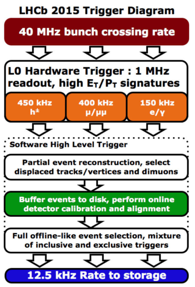
Trigger
- Decisions based on the detector responses to reduce the event rate on storage.
-
Divided in three stages:
- One hardware level and two software levels.
The LHC can provide a bunch crossing every 25ns \(\Rightarrow\) How is decided what to save?
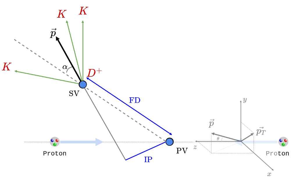
Main properties measured at LHCb
Experimental Setup
Sebastian Ordoñez-Soto
January 24th, 2025
-
Kinematic
- Momentum \(\vec{p} = (p_{x},p_{y},p_{z})\), pseudorapidity \(\eta = -\ln{(\tan{(\frac{\theta}{2})})} \), transverse momentum \(p_{T}\), direction angle \(\alpha\) ...
-
Topological
- Primary vertex (PV), Secondary vertex (SV), Flight distance (FD), Impact parameter (IP), Vertex \(\chi^{2}\), Track \(\chi^{2}\)/dof, ...
-
Identification
- Probability of a final state candidate being a kaon \(\Rightarrow\) \(\text{Prob}(K^{\pm})\)
The LHCb detector measures physical properties of particles -variables- resulting from \(pp\) collisions.
Relevant variables for the \(D^{+}\rightarrow 3K\) analysis
Experimental Setup
Sebastian Ordoñez-Soto
January 24th, 2025
Key points for the \(D^{+}\rightarrow 3K\) analysis:
-
Three charged tracks in the final state identified as kaons
- Requires good-quality tracks and PID.
- Tracks must form a good-quality SV, detached from the PV
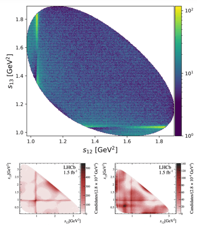
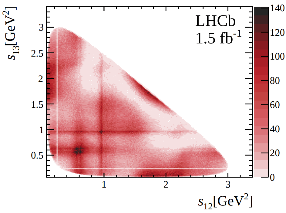
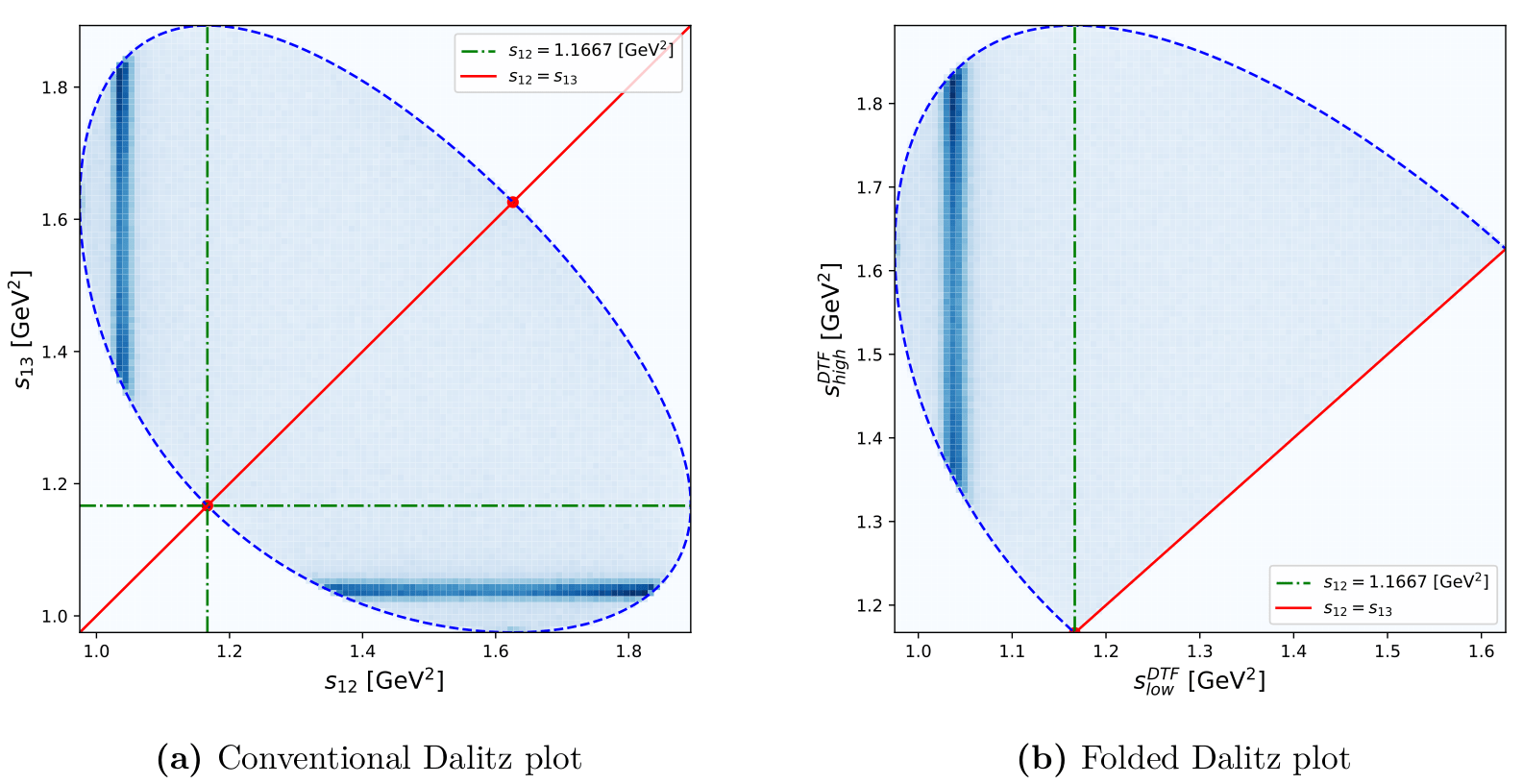
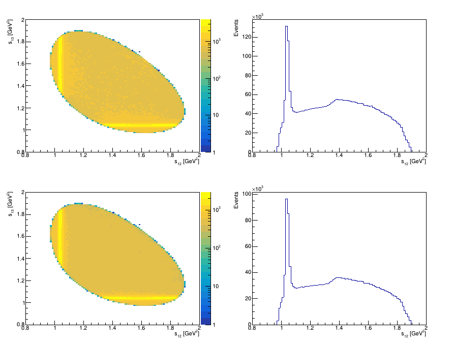
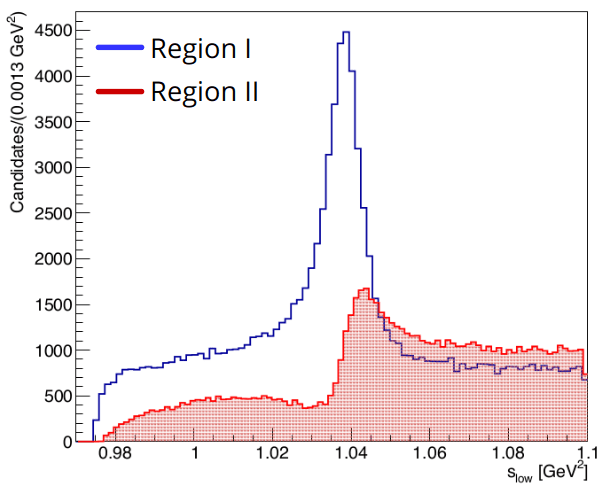
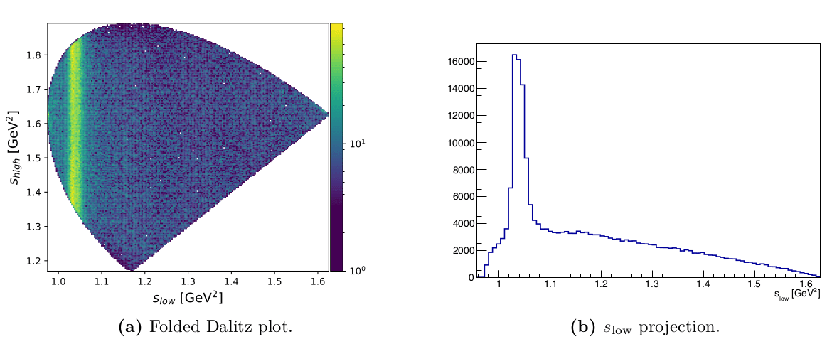
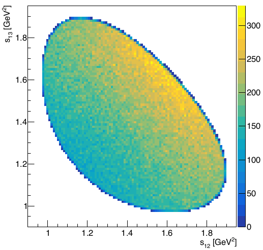
Dalitz plot folded
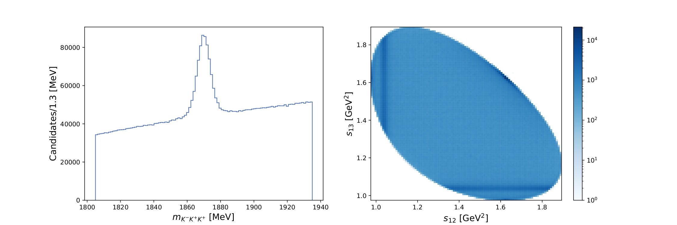
Invariant mass of the three kaons and Dalitz plot
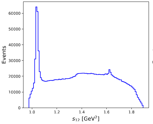
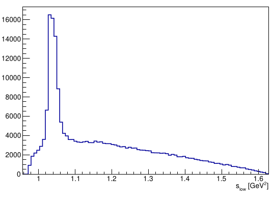
Main variables used:
- \(m_{K^{-}K^{+}K^{+}}\) \(\Rightarrow\) Invariant mass of the kaon candidates.
- \(s_{12}\) and \(s_{13}\) \(\Rightarrow\) Dalitz variables.
- \(s_{\text{low}}\) and \(s_{\text{high}}\) \(\Rightarrow\) Dalitz plot folded variables.
Amplitude Analysis of the \(D^{+}\rightarrow K^{-}K^{+}K^{+}\) decay
Analysis Strategy
Sebastian Ordoñez-Soto
January 24th, 2025
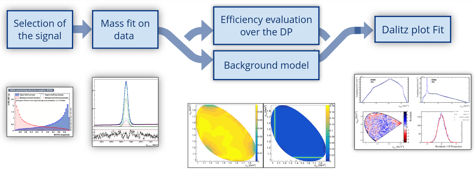
Amplitude Analysis of the \(D^{+}\rightarrow K^{-}K^{+}K^{+}\) decay
| Selection of the signal |
| Efficiency evaluation over the DP |
| Background model |
| Dalitz plot Fit |
| Mass fit on data |
The analysis consists of mainly five stages, from the signal selection to the final Dalitz plot fit.
Sebastian Ordoñez-Soto
January 24th, 2025
Amplitude Analysis of the \(D^{+}\rightarrow K^{-}K^{+}K^{+}\) decay
Analysis Strategy

Pre-selection and vetoes
Sebastian Ordoñez-Soto
January 24th, 2025
Amplitude Analysis of the \(D^{+}\rightarrow K^{-}K^{+}K^{+}\) decay
-
Pre-selection
- Rule out obvious uninteresting events.
-
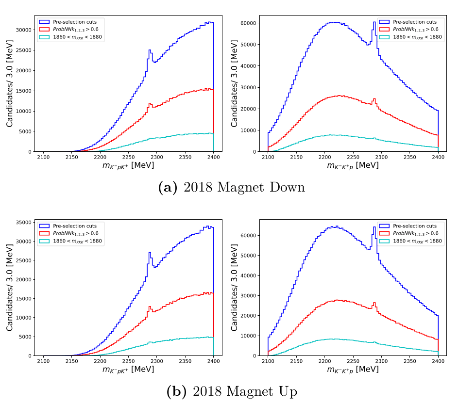
Specific backgrounds \(\Rightarrow\) Generate structures in the DP.
-
Charm backgrounds
- MisID \(\Rightarrow\) \(\Lambda_{c}\rightarrow K^{-}K^{+}p\) and \(\Lambda_{c}\rightarrow K^{-}\pi^{+}p\)
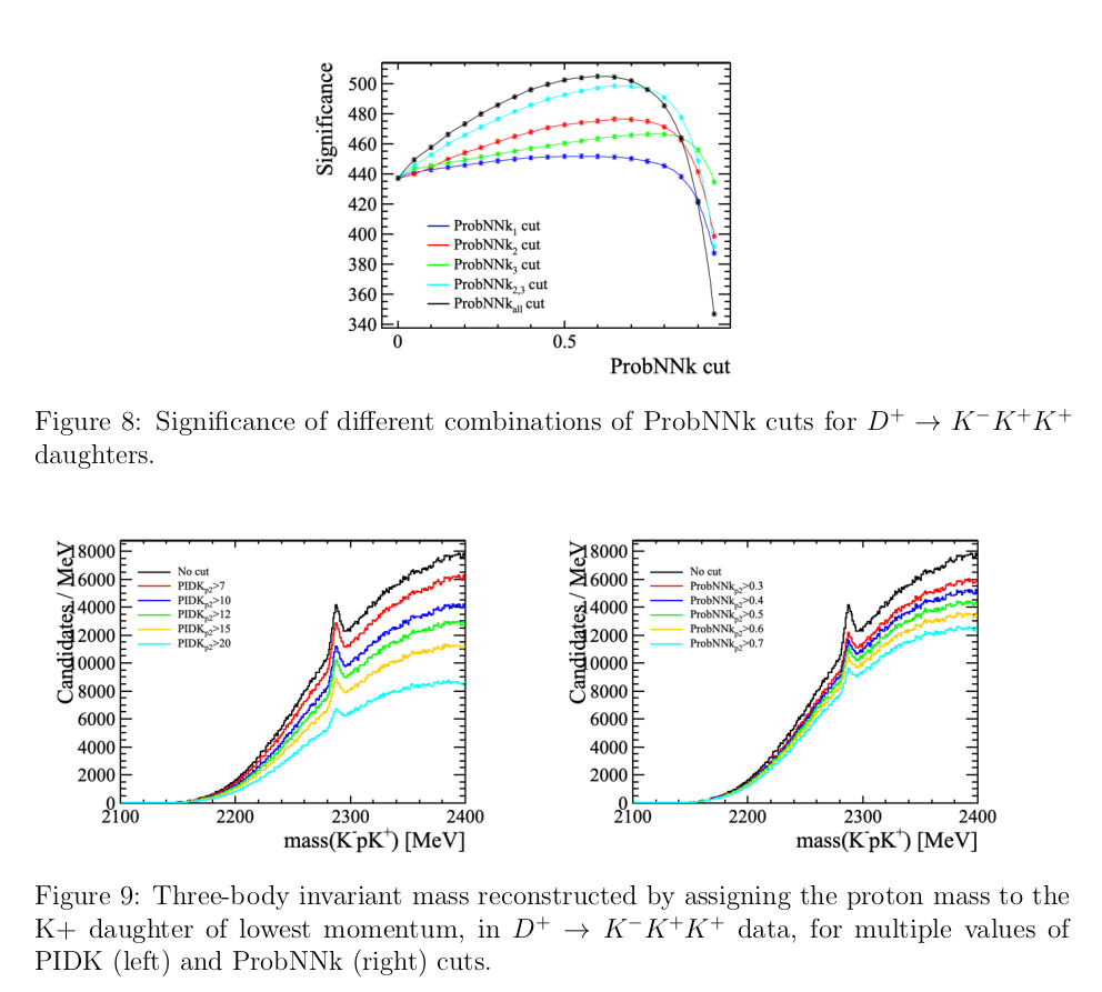
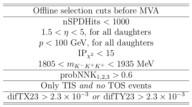
- Vetoes on PID variables: \(\text{Prob}(K^{\pm})\)\(_{1,2,3}>0.6\)
-
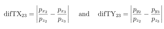
Clone tracks
- Two tracks related to a single particle due to spatial proximity.
- Difference in the slope between the two tracks.
-
Charm backgrounds
-
Combinatorial background \(\Rightarrow\) No structures in the DP.
- Random combination of three kaon-like tracks.
After the trigger selection, the background levels in the data samples are still elevated.
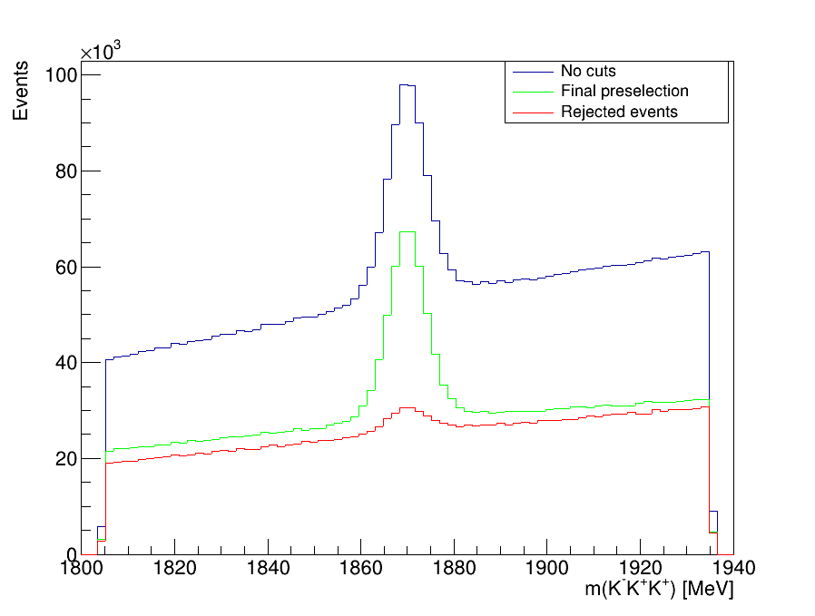

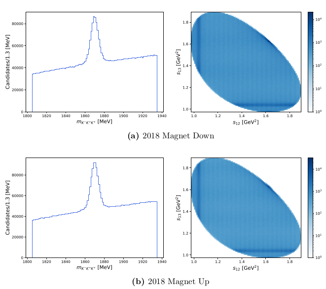
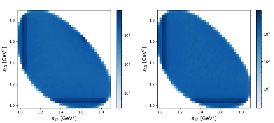
Invariant mass before and after pre-selection
DP before and after pre-selection
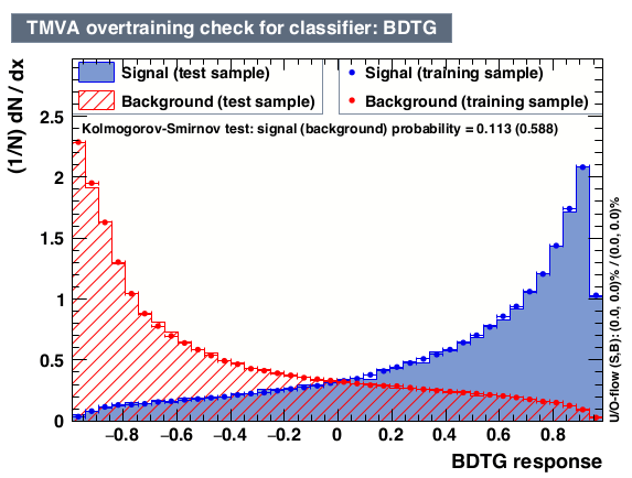
Multivariate Analysis selection
Sebastian Ordoñez-Soto
January 24th, 2025
Amplitude Analysis of the \(D^{+}\rightarrow K^{-}K^{+}K^{+}\) decay
-
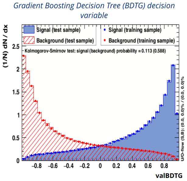
Training and Testing
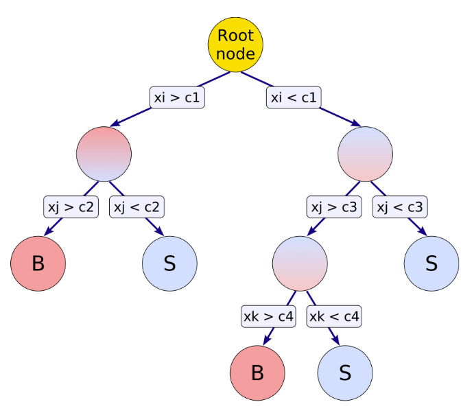
- A BDTG is trained with labeled samples: signal and bkg.
- A set of discriminating variables are provided.
-
Result: probabilities of being either signal or bkg.
- Decision variable \(\Rightarrow\) valBDTG
-
Application
- The decision variable is applied to an unlabeled sample.
-
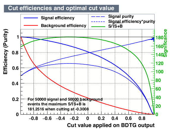
Evaluation of FoM \(\Rightarrow\) Purity
- Optimization of the amount of signal candidates.
Use of machine learning techniques to reduce the amount of the remaining background.
\text{Purity}_{i} = \frac{S_{i}}{S_{i}+B_{i}} = \frac{N_{0}^{\text{sig}}\epsilon_{i}^{\text{sig}}}{N_{0}^{\text{sig}}\epsilon_{i}^{\text{sig}}+N_{i}^{\text{bkg}}}
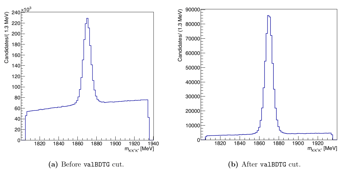
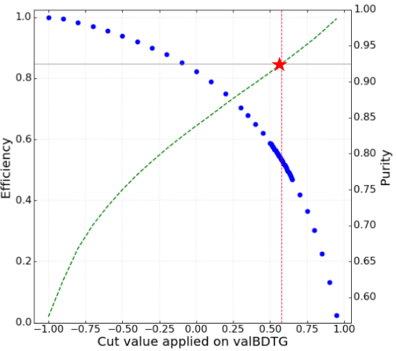
A cut at valBDTG> 0.575 achieves a purity of 92.5% within the signal region with a signal efficiency of ~54%.
Sebastian Ordoñez-Soto
January 24th, 2025
Amplitude Analysis of the \(D^{+}\rightarrow K^{-}K^{+}K^{+}\) decay
Analysis Strategy
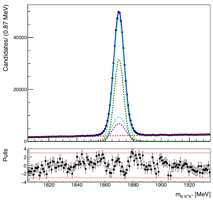
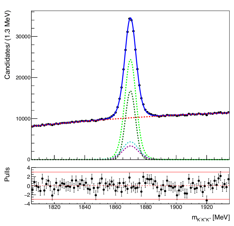
Invariant mass fit of the \(K^{-}K^{+}K^{+}\) spectrum
Sebastian Ordoñez-Soto
January 24th, 2025
Amplitude Analysis of the \(D^{+}\rightarrow K^{-}K^{+}K^{+}\) decay
The \(K^{-}K^{+}K^{+}\) mass spectrum is fitted to determine:
- Final signal region \(\mu\pm 2\sigma_{eff}\)
- Fraction of signal (\(f_{sig}\)) and background (\(f_{bkg}\))
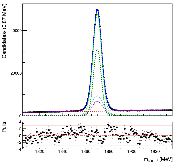
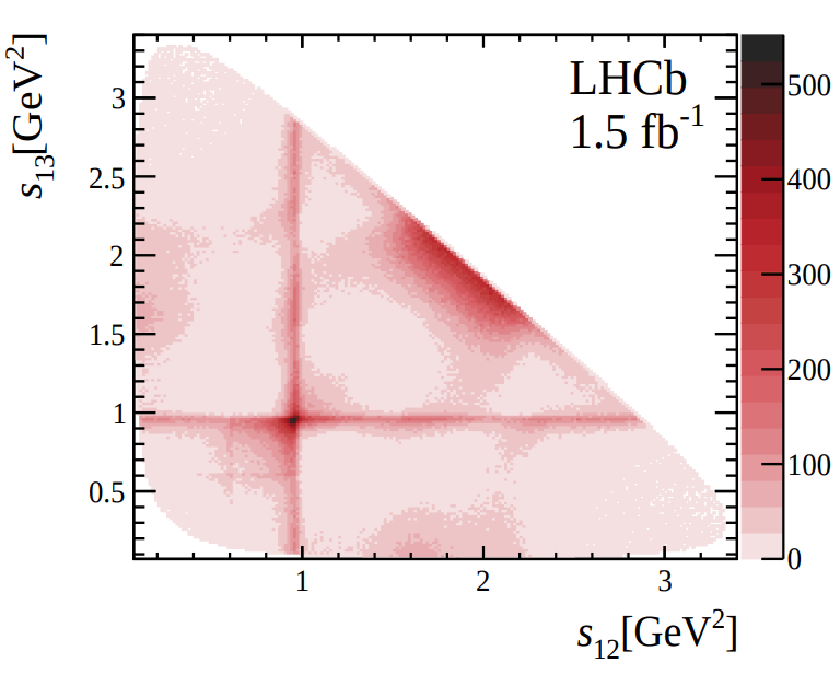
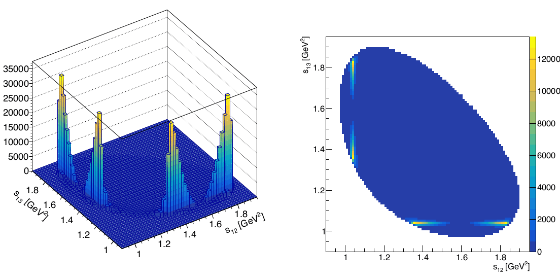
The number of signal and bkg. events within the signal region yields \(512202\pm 745\) and \(42383\pm 225\), resp.
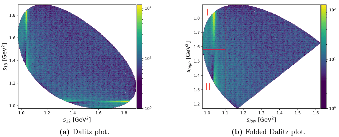
Dalitz plot distribution of selected data.
\([1861.94,1878.3]\) MeV
Sebastian Ordoñez-Soto
January 24th, 2025
Amplitude Analysis of the \(D^{+}\rightarrow K^{-}K^{+}K^{+}\) decay
Analysis Strategy
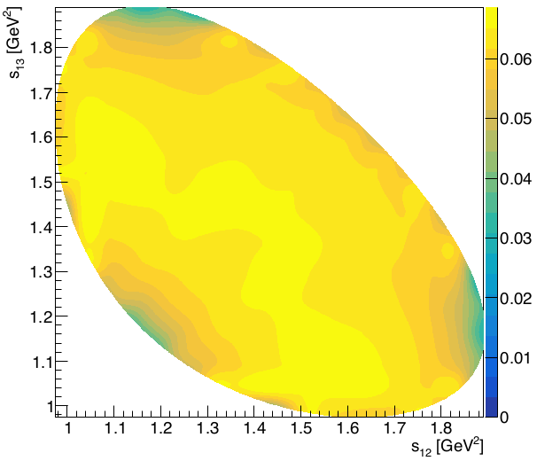
Efficiency evaluation over the DP
Sebastian Ordoñez-Soto
January 24th, 2025
Amplitude Analysis of the \(D^{+}\rightarrow K^{-}K^{+}K^{+}\) decay
-
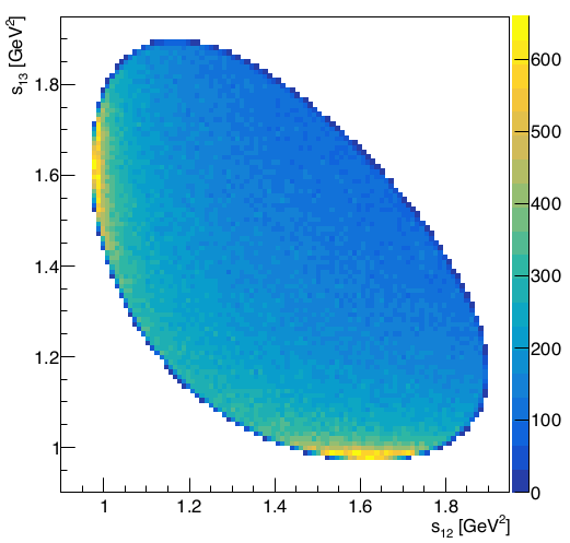
Efficiency map \(\epsilon(s_{12},s_{13})\)
- Determined from phase space MC events -corrected- passed through all the selection.
-
The efficiency histogram (15x15 bins) is smoothed resulting in a high-resolution histogram.
- This histogram will weight the signal and background PDFs in the DP fit.
The efficiency impacts 3 regions at the DP boundary \(\Rightarrow\) Does not compromise significantly the region near threshold.
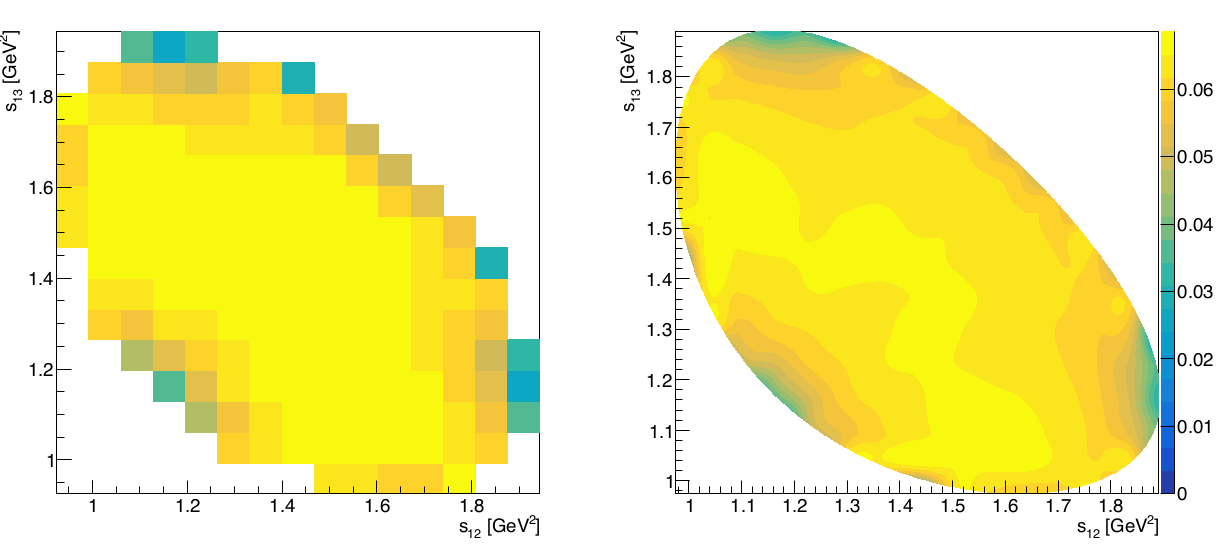
The binning is a source of systematic uncertainty
\(\epsilon(s_{12},s_{13})\)
It is necessary to account for the variation of the detection efficiency across the phase space.
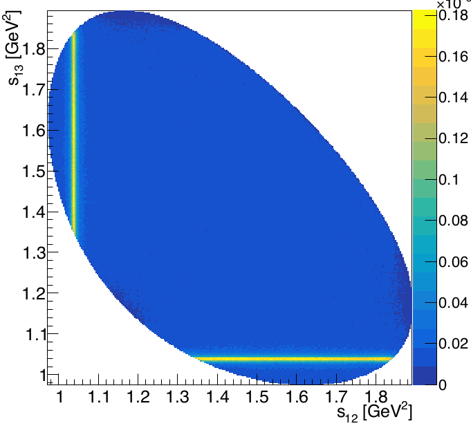
Background Model
Sebastian Ordoñez-Soto
January 24th, 2025
Amplitude Analysis of the \(D^{+}\rightarrow K^{-}K^{+}K^{+}\) decay
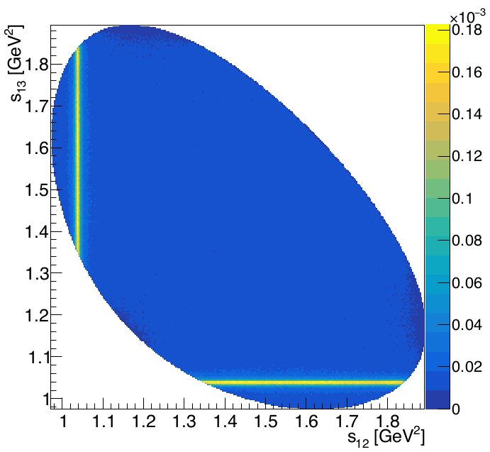
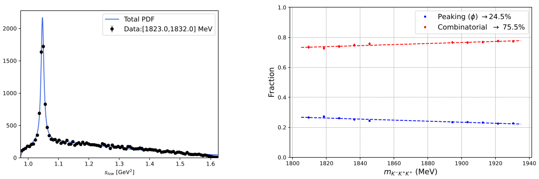
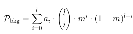
- Inspection of the side-bands suggest two components: peaking \(\phi\)-like [1] and a smooth Phase Space [2].
-
Background fractions
- The side-bands are divided into slices of 9 MeV \(\Rightarrow\) \(s_{low}\) fit to get the fractions of each component.
-
Extrapolation of the fractions to the signal region \(\Rightarrow\) [1]: \(24.53\pm 0.14\)% and [2]: \(75.47\pm 0.11\)%
- A histogram is built from a simulated sample with these relative proportions \(\Rightarrow\) \(\mathcal{B}_{PDF}(s_{12},s_{13})\)
\(\mathcal{B}_{PDF}(s_{12},s_{13})\)
The contribution of background needs to be accounted for in the DP fit.
The model is a source of systematic uncertainty
Sebastian Ordoñez-Soto
January 24th, 2025
Amplitude Analysis of the \(D^{+}\rightarrow K^{-}K^{+}K^{+}\) decay
Analysis Strategy
Dalitz plot fit to data
Sebastian Ordoñez-Soto
January 24th, 2025
Amplitude Analysis of the \(D^{+}\rightarrow K^{-}K^{+}K^{+}\) decay
The isobar parameters (\(a_{k}\), \(\delta_{k}\)) for each channel are floated in the fit as well as the fit fractions \(FF_{k}\).
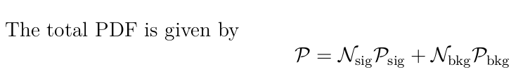
\boxed{\mathcal{L} = \prod^{N_{\text{cand}}}_{i=1} f_{\text{sig}}\cdot\mathcal{S}_{\text{PDF}}(s_{12}^{i},s_{13}^{i}) + f_{\text{bkg}}\cdot \mathcal{B}_{\text{PDF}}(s_{12}^{i},s_{13}^{i})} \Rightarrow \boxed{\text{FCN} = -2 \ln\mathcal{L}}
-
Normalised signal PDF
- \(\mathcal{S}_{\text{PDF}}(s_{12}^{i},s_{13}^{i}) = \frac{1}{N_{\text{S}}}|\mathcal{M}(s_{12}^{i},s_{13}^{i})|^{2}\epsilon(s_{12}^{i},s_{13}^{i})\) \(\Rightarrow\) Decay amplitude \(\mathcal{M}\) from Isobar Model (IM)
- Signal and background fractions (\(f_{sig}\) & \(f_{bkg}\)) \(\Rightarrow\) From mass fit to data
- Background and efficiency maps (\(\mathcal{B}_{PDF} (s_{12},s_{13})\) & \(\epsilon (s_{12},s_{13})\)) \(\Rightarrow\) Input models from simulations
An unbinned maximum-likelihood fit is applied to the final Dalitz plot distribution.
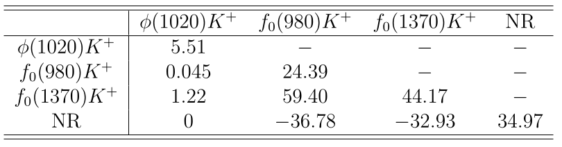
- Fit fractions \(\Rightarrow\)Rough approximation of the proportion of a resonance within a model.
\boxed{\text{FF}_{ij} = \frac{\iint_{DP} \,ds_{12}\,ds_{13} \hspace{1mm}2\mathcal{Re}|c_{i}c_{j}^{*}M_{i}M_{j}^{*}|^{2}}{\iint_{DP}\,ds_{12}\,ds_{13} \hspace{1mm}|\sum_{k}c_{k}M_{k}(s_{12},s_{13})|^{2}}}
\boxed{\text{FF}_{k} = \frac{\iint_{DP} \,ds_{12}\,ds_{13} \hspace{1mm}|c_{k}M_{k}(s_{12},s_{13})|^{2}}{\iint_{DP}\,ds_{12}\,ds_{13} \hspace{1mm}|\sum_{i}c_{i}M_{i}(s_{12},s_{13})|^{2}}.}
Interference fit fractions
Signal models
Sebastian Ordoñez-Soto
January 24th, 2025
Amplitude Analysis of the \(D^{+}\rightarrow K^{-}K^{+}K^{+}\) decay
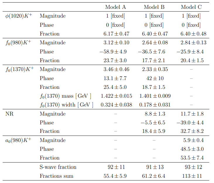
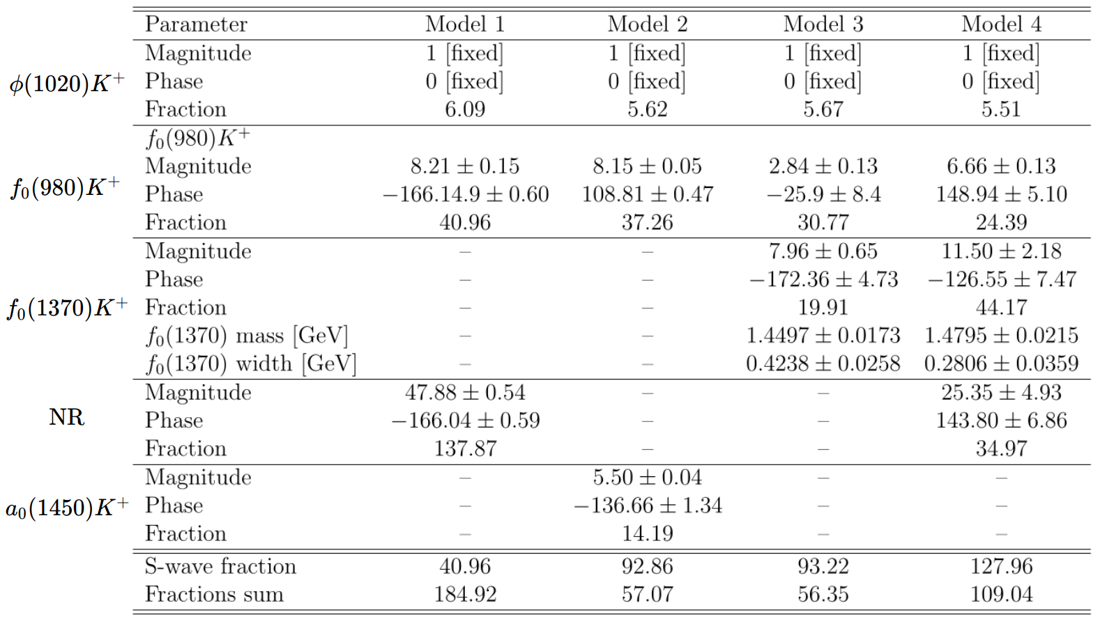
Four models are considered, all containing \(\mathcal{S}\)-wave components:
- Model 1: \(\phi(1020)\) + \(f_{0}(980)\) and a NR amplitude.
- Model 2: \(\phi(1020)\) + \(f_{0}(980)\) and the \(a_{0}(1450)\) resonance.
- Model 3: \(\phi(1020)\) + \(f_{0}(980)\) and the \(f_{0}(1370)\) scalar.
- Model 4: \(\phi(1020)\) + \(f_{0}(980)\) + \(f_{0}(1370)\) scalar and a NR amplitude. \(\Rightarrow\) Baseline model
\(\phi K^{+}\) mode is chosen as reference \(\Rightarrow\) Fixed: \(a_{\phi} = 1\) and \(\delta_{\phi} = 0°\)
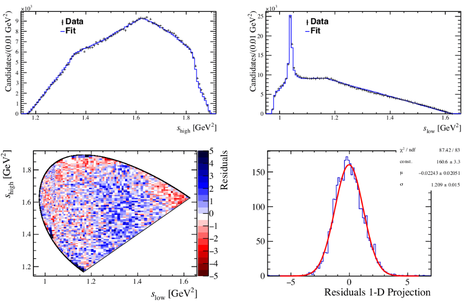
Results of Dalitz plot fits
Sebastian Ordoñez-Soto
January 24th, 2025
Amplitude Analysis of the \(D^{+}\rightarrow K^{-}K^{+}K^{+}\) decay
-
Goodness-of-fit
-
Normalized residuals
- \(\boxed{\Delta_{i} = \frac{N_{\text{fit}}^{i}-N_{\text{obs}}^{i}}{\sigma_{i}}}\)
-
Test statistic \(\chi^{2}\)/ndof
- \(\boxed{\chi^{2} = \sum_{i=1}^{n_{\text{b}}}\chi_{i}^{2} = \sum_{i=1}^{n_{\text{b}}} \frac{(N_{\text{fit}}^{i}-N_{\text{obs}}^{i})^{2}}{\sigma_{i}^{2}}}\)
-
Normalized residuals
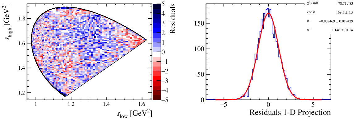
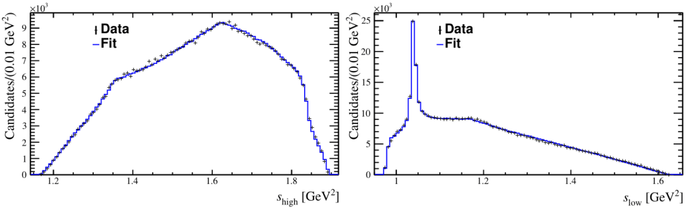
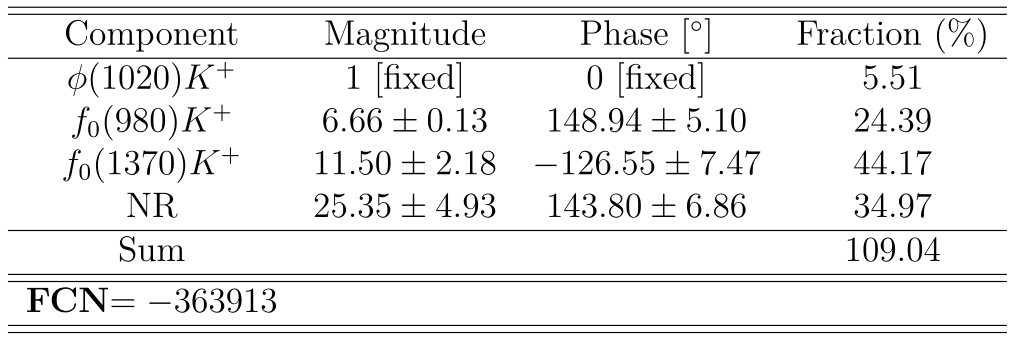
Results for the baseline model
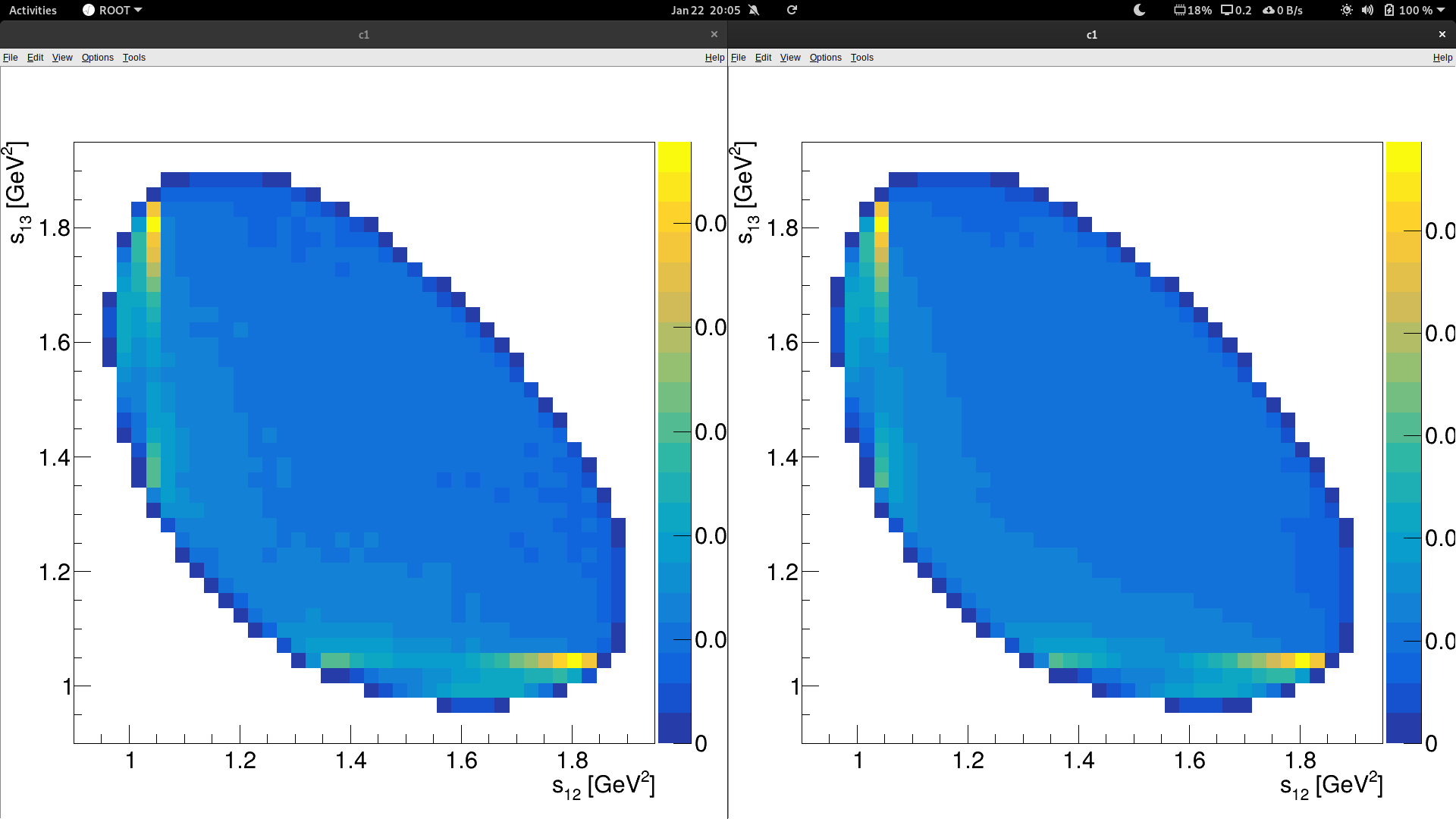
Comparison between data DP and a baseline model simulation
Data
Simulation
Results of Dalitz plot fits
Sebastian Ordoñez-Soto
January 24th, 2025
Amplitude Analysis of the \(D^{+}\rightarrow K^{-}K^{+}K^{+}\) decay
- The \(\mathcal{S}\)-wave is the most relevant contribution for the description of the \(D^{+}\rightarrow K^{-}K^{+}K^{+}\) decay.
- The interference between the \(\mathcal{S}\)-wave components is high. A small interference with the \(\phi(1020)\) is observed in all models.
- It is crucial for the description the inclusion of a resonance in the high-mass region, such as the \(f_{0}(1370)\).
https://arxiv.org/pdf/1902.05884
Previous LHCb results
DP fit systematic uncertainties
Sebastian Ordoñez-Soto
January 24th, 2025
Amplitude Analysis of the \(D^{+}\rightarrow K^{-}K^{+}K^{+}\) decay
-
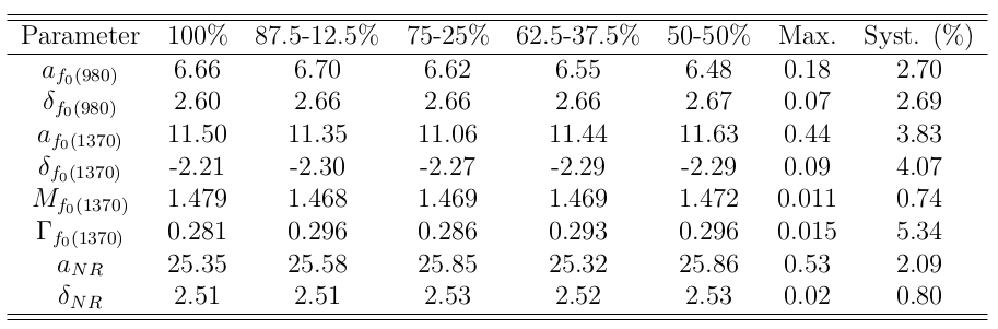
Background modeling \(\Rightarrow\) the smooth component may still contain a contribution from \(f_{0}(980)\)
- Fits are performed varying percentages of \(f_{0}(980)K^{+}\) alongside the phase space component.
-
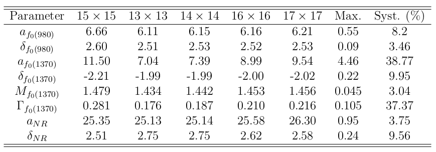
Binning scheme of the efficiency map \(\Rightarrow\) There is no an obvious selection of the binning.
- Fits are carried out with different binning for the efficiency histogram.
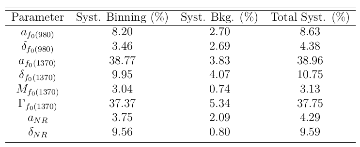
The main sources of syst. uncertainties are the background model and the binning scheme of the efficiency map.
Total systematic uncertainties (%)
- Uncertainties associated with the background modeling are small.
-
Most parameters are robust under changes to the binning scheme.
- Those related to the \(f_{0}(1370)\) resonance, are highly sensitive.
Summary
Summary and conclusions
Conclusion
Sebastian Ordoñez-Soto
January 24th, 2025
-
A Dalitz plot analysis of the doubly Cabibbo-suppressed \(D^{+}\rightarrow K^{-}K^{+}K^{+}\) decay was performed, using the largest dataset collected to date.
-
The decay is largely dominated by S-wave components, with an additional contribution from the \(\phi(1020)\) (~5.5%) and significant interference among the different components.
-
Difficulty in disentangling individual S-wave components due to the limited phase space, lack of structures beyond \(\phi(1020)\), and the \(f_{0}(980)\) lying below the \(K^{+}K^{-}K^{-}\) threshold.
-
The findings align with other three-body decays of \(D^{+}\) and \(D_{s}^{+}\), while exploring alternative approaches for describing the S-wave within the LHCb collaboration.
Thank you for your attention!
Back up
Mesons
Scientific context
Sebastian Ordoñez-Soto
January 24th, 2025
- Type of hadronic subatomic particle (~\(10^{-15}\)m) composed of an equal number of quarks and antiquarks, bound together by the strong interaction.
-
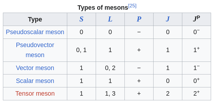
Mesons are classified according to their quark content, total angular momentum, parity and various other properties
-
Because mesons are made of one quark and one antiquark, they are found in triplet and singlet spin states
The \(D\) mesons are the lightest particle containing charm quarks.
\(D^{+}\) mass: 1869.62\(\pm\)0.20 MeV
Light meson spectroscopy
Scientific context
Sebastian Ordoñez-Soto
January 24th, 2025
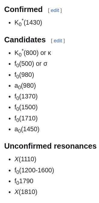
- A scalar meson is a meson with total spin 0 and even parity (usually noted as \(J^{P}=0^{+}\)).
-
Groups: The light (unflavored) scalar mesons may be divided into three groups.
- mesons having a mass below 1 GeV
- mesons having a mass between 1 GeV and 2 GeV
- other radially-excited unflavored scalar mesons above 2 GeV
- The lightest scalar mesons have been interpreted by some theorists to be possible tetraquark or meson-meson "molecule" states.
SM review
Scientific context
Sebastian Ordoñez-Soto
January 24th, 2025
Scattering review
Scientific context
Sebastian Ordoñez-Soto
January 24th, 2025
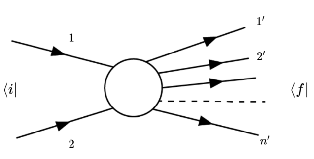
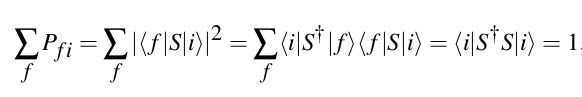
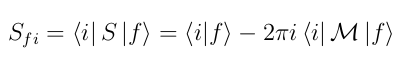
Given an initial set of well defined states |i⟩ that are allowed to interact under fundamental interactions, which are going to be the observable results, i.e. the final states |f ⟩
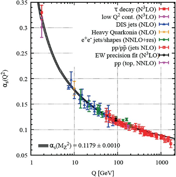
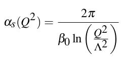
- Advances have been done in order to get a theory of strong interactions, resulting in QCD.
- The interaction term has an associated coupling constant, g , that determines its strength.
- It was found that coupling is energy-scale dependent:
Behind DP
Sebastian Ordoñez-Soto
January 24th, 2025
Scientific context
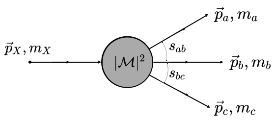
- The decay rate (Γ) is given by the number of decays per unit of time divided by the number of initial state particles present
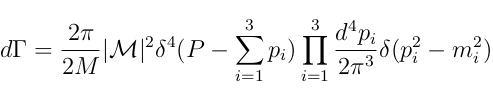
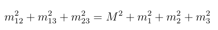
- The constraints imposed for N=3 final state of spin-0 particles reveal that only 2 of the 12 variables are independent variables.
- Energy and momentum conservation reduce to 5. The spin-0 particles are restricted to the same plane where orientation is arbitrary, thus reducing to 2 d.o.f
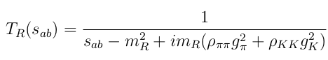
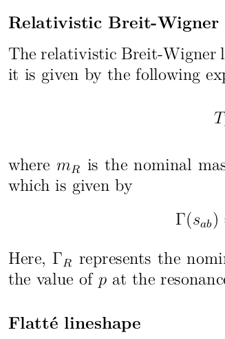
Isobar Model
Sebastian Ordoñez-Soto
January 24th, 2025
Scientific context

Isobar Model
Sebastian Ordoñez-Soto
January 24th, 2025
Scientific context
LHC
Experimental Setup
Sebastian Ordoñez-Soto
January 24th, 2025
LHC
Experimental Setup
Sebastian Ordoñez-Soto
January 24th, 2025

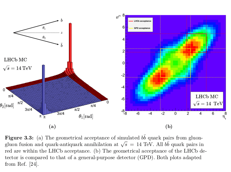
LHCb geometry motivtion
Experimental Setup
Sebastian Ordoñez-Soto
January 24th, 2025
Trigger, preselection and vetoes
Sebastian Ordoñez-Soto
January 24th, 2025
Amplitude Analysis of the \(D^{+}\rightarrow K^{-}K^{+}K^{+}\) decay
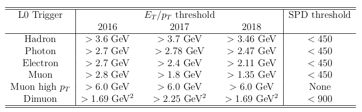
Hardware Trigger
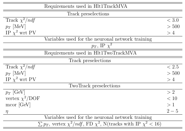
Software trigger (I)
Trigger, preselection and vetoes
Sebastian Ordoñez-Soto
January 24th, 2025
Amplitude Analysis of the \(D^{+}\rightarrow K^{-}K^{+}K^{+}\) decay
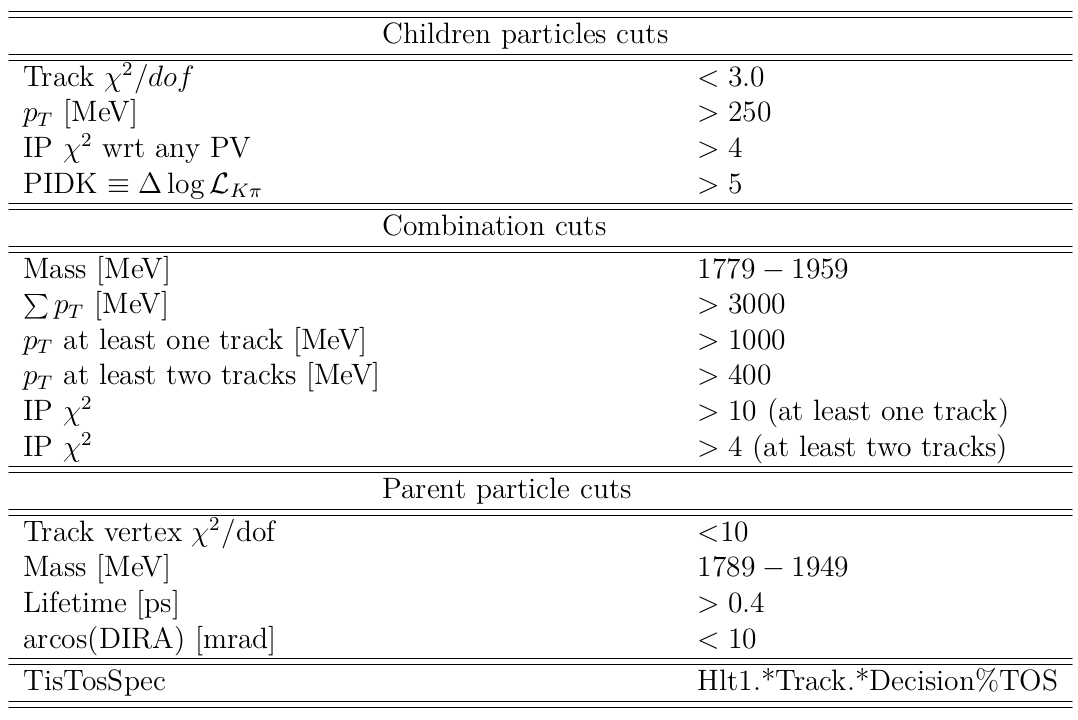
Selection criteria corresponding to the trigger systmem which selects the \(D\rightarrow 3K\) candidates.
Pre-selection
Sebastian Ordoñez-Soto
January 24th, 2025
Amplitude Analysis of the \(D^{+}\rightarrow K^{-}K^{+}K^{+}\) decay
Pre-selection
Sebastian Ordoñez-Soto
January 24th, 2025
Amplitude Analysis of the \(D^{+}\rightarrow K^{-}K^{+}K^{+}\) decay
Pre-selection
Sebastian Ordoñez-Soto
January 24th, 2025
Amplitude Analysis of the \(D^{+}\rightarrow K^{-}K^{+}K^{+}\) decay

Offline selection before MVA
Sebastian Ordoñez-Soto
January 24th, 2025
Amplitude Analysis of the \(D^{+}\rightarrow K^{-}K^{+}K^{+}\) decay
Mass spectrum fits to pre-selected samples
Sebastian Ordoñez-Soto
January 24th, 2025
Amplitude Analysis of the \(D^{+}\rightarrow K^{-}K^{+}K^{+}\) decay
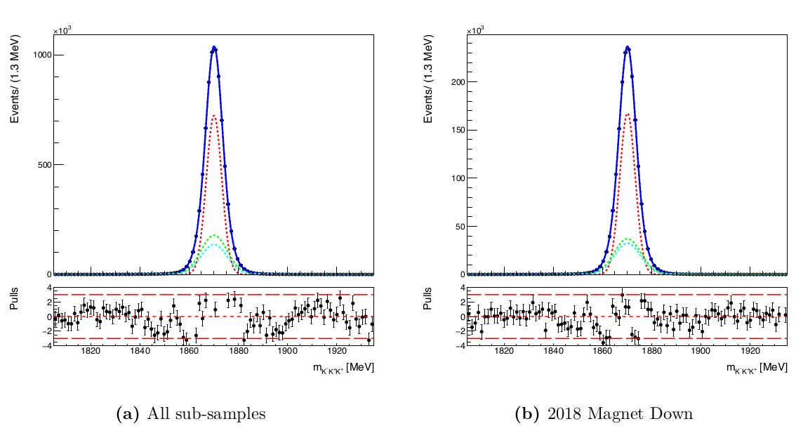
Data
Simulation
Correction of the simulation data
Sebastian Ordoñez-Soto
January 24th, 2025
Amplitude Analysis of the \(D^{+}\rightarrow K^{-}K^{+}K^{+}\) decay
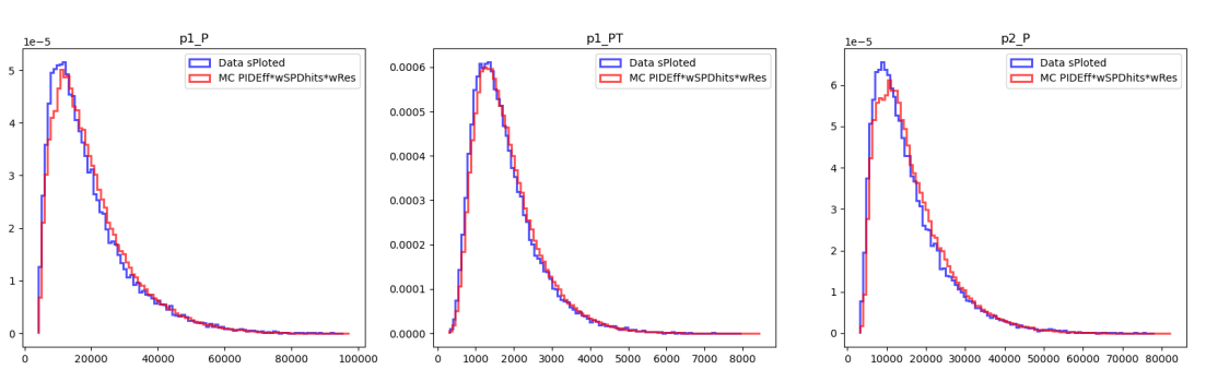
The goal of MC data is to replicate the observed signal, though discrepancies may require additional corrections \(\Rightarrow\) Incorporation of weights (\(\omega\)):
-
PID corrections (\(\omega_{PID}\)) \(\Rightarrow\) MC
- Calibration samples are used to provide an efficiency for each event for a given PID cut.
-
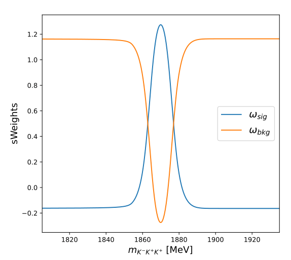
Signal weights (\(\omega_{sig}\)) \(\Rightarrow\) Data
- The sPlot technique is employed to obtain background-subtracted data.
-
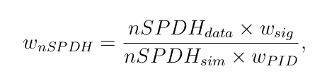
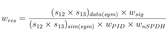
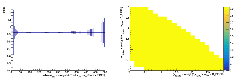
Kinematics and dynamics (\(\omega_{nSPDH}\) and \(\omega_{res}\)) \(\Rightarrow\) MC
- A weight is obtained for MC candidates in order to equalize the distributions of the number of SPD hits
- A weight aims to account for the dynamics (resonant structure) in the Dalitz plot.
-
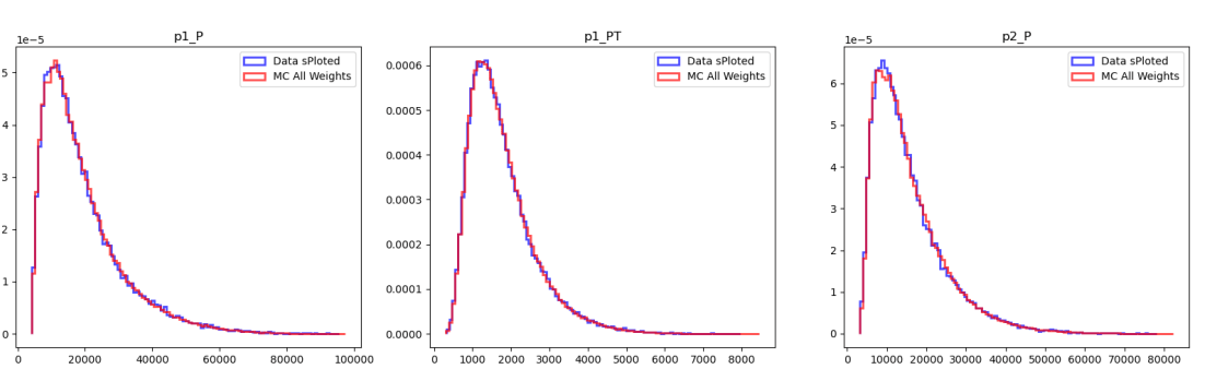
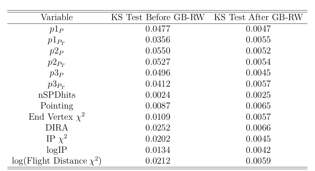
Gradient Boosted Reweighter (\(\omega_{GB}\)) \(\Rightarrow\) MC
- Machine learning algorithm used to match data and simulated data distributions.
- Ensures that all the MC variables that will be used in next steps coincide with those of the data.
Data ready for Multivariate Analysis selection to fight against the remaining combinatorial background!
Sebastian Ordoñez-Soto
January 24th, 2025
Amplitude Analysis of the \(D^{+}\rightarrow K^{-}K^{+}K^{+}\) decay
Correction of the simulation data
Sebastian Ordoñez-Soto
January 24th, 2025
Amplitude Analysis of the \(D^{+}\rightarrow K^{-}K^{+}K^{+}\) decay
Correction of the simulation data
Before GB reweight
After GB reweight
Sebastian Ordoñez-Soto
January 24th, 2025
Amplitude Analysis of the \(D^{+}\rightarrow K^{-}K^{+}K^{+}\) decay
Correction of the simulation data
Sebastian Ordoñez-Soto
January 24th, 2025
Amplitude Analysis of the \(D^{+}\rightarrow K^{-}K^{+}K^{+}\) decay
MVA
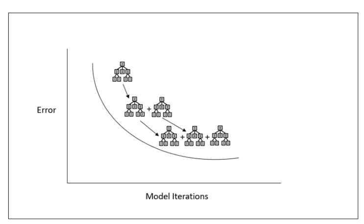
The gradient descent optimization.
An example of a Decision Tree
Sebastian Ordoñez-Soto
January 24th, 2025
Amplitude Analysis of the \(D^{+}\rightarrow K^{-}K^{+}K^{+}\) decay
MVA
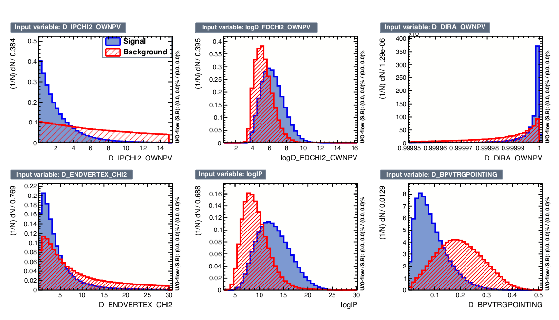
Discriminant input variables for training of the BDTG classifier
Sebastian Ordoñez-Soto
January 24th, 2025
Amplitude Analysis of the \(D^{+}\rightarrow K^{-}K^{+}K^{+}\) decay
MVA
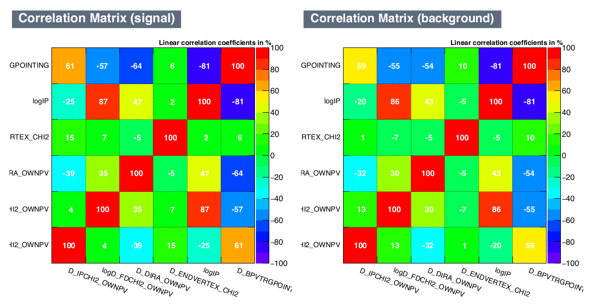
Linear correlation matrices
Sebastian Ordoñez-Soto
January 24th, 2025
Amplitude Analysis of the \(D^{+}\rightarrow K^{-}K^{+}K^{+}\) decay
MVA
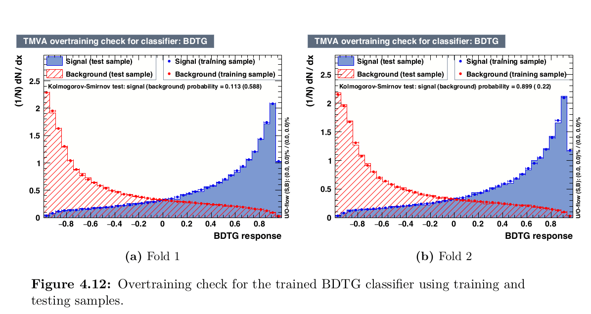
Over-training check
Sebastian Ordoñez-Soto
January 24th, 2025
Amplitude Analysis of the \(D^{+}\rightarrow K^{-}K^{+}K^{+}\) decay
MVA
Evaluation of the performance of the BDTG classifier
Sebastian Ordoñez-Soto
January 24th, 2025
Amplitude Analysis of the \(D^{+}\rightarrow K^{-}K^{+}K^{+}\) decay
MVA
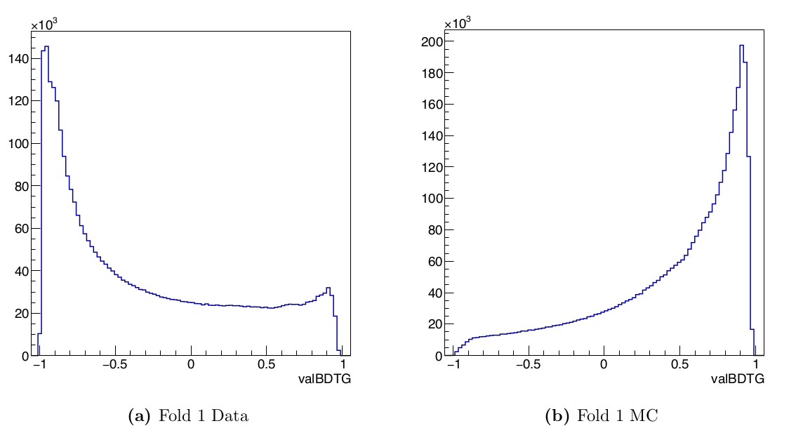
Distributions of the predicted BDTG decision variable for both data and
simulated samples
Sebastian Ordoñez-Soto
January 24th, 2025
Amplitude Analysis of the \(D^{+}\rightarrow K^{-}K^{+}K^{+}\) decay
Invariant mass fit
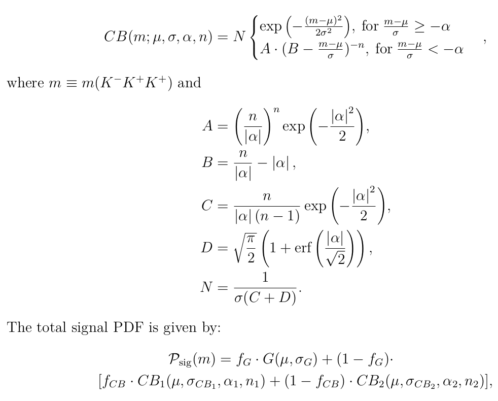
Signal PDF, Background PDF and Total PDF
Systematic uncertainties
Sebastian Ordoñez-Soto
January 24th, 2025
Amplitude Analysis of the \(D^{+}\rightarrow K^{-}K^{+}K^{+}\) decay
- Background modeling \(\Rightarrow\) the smooth component may still contain a contribution from \(f_{0}(980)\)
- Binning scheme of the eff. map \(\Rightarrow\) There is no a straightforward selection of binning.
The main sources come from the background model and the binning scheme of the efficiency map.
Systematic uncertainties (%) due to the bkg. modeling.
Systematic uncertainties (%) due to the binning scheme.
Total systematic uncertainties (%)
Master Thesis Defense
By Sebastian Ordoñez


