Study of the resonant structure in the decay of charmed mesons
\(D^{+}\longrightarrow K^{-}K^{+}K^{+}\)
CERN Summer Student Programme
Sebastian Ordoñez
jsordonezs@unal.edu.co
Supervisor: Alberto C. dos Reis
9th of July 2021
Motivation
- The theoretical treatment of weak decays of charm mesos is rather difficult and the typical approaches, chiral perturbation theory and heavy-quark tools, are not directly applicable.
- Phenomenological models have been developed, e.g. the Multi-Meson Model. These models are our best try for describing \(c\) meson decays up to date.
Weak decay of charmed mesons
For those models the knowledge of branching fractions and resonant structures are key inputs!
Current status within the LHCb collaboration (as far as I know)
Mainly summarized in two papers:
- Measurement of the branching fractions: https://arxiv.org/pdf/1810.03138v2.pdf
- Dalitz plot analysis of the \(D^{+}\longrightarrow K^{-}K^{+}K^{+}\): https://arxiv.org/pdf/1902.05884.pdf
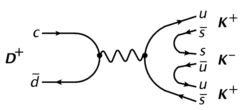
Amplitude Analysis of the \(D^{+}\longrightarrow K^{-}K^{+}K^{+}\)
The amplitude analysis is performed using two models: the traditional isobar model and the most interesting one, the Multi-Meson Model alias Triple-M.
- Isobar Model: The decay amplitude is a coherent sum of resonant and non-resonant amplitudes. It is well known to arise some physical issues, e.g. unitarity violation. Its fit parameters are complex constants without any physical meaning.
- Multi-Meson Model: Derived from an effective chiral Lagrangian with resonances. One of its more fundamental features is that it includes the effects of coupled channels in the Final State Interactions (FSI).
Big picture of a three-body decay as described by the Triple-M:
\(c\) quark decay
Formation of the mesons
Final State Interactions
Additional motivation: \(K^{-}K^{+}\) scattering amplitudes
Three-body decays of \(D\) mesons into kaons \(K\) and pions \(\pi\) are interesting laboratories for light-meson spectroscopy.
It is neccesary to isolate the physics of two-body systems from the rich dynamics of three-body decays!
Candidate selection
It is required:
- Three charged particles identified as kaons according to the particle identification (PID) criteria
- These particles must form a good-quality decay vertex, detached from the PV.
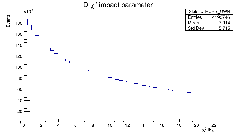
The most important variables used for selecting candidates are:
- Flight distance (FD): ditance between the PV and the \(D^{+}\) decay vertex.
- Impact parameter (IP) of the \(D^{+}\) candidate.
- The angle between the reconstructed \(D^{+}\) momentum vector and the vector containing the PV to the decay vertex
- The \(\chi^{2}\) of the \(D^{+}\) decay vertex fit.
- The distance of the closest approach between any two final-state tracks.
- The momentum, the transverse momentum and the \(\chi^{2}_{IP}\) of the \(D^{+}\) candidate and of its decay products.
- The invariant mass of the \(D^{+}\) candidate is required to be within the interval 1820-1920 MeV
Variables employed for the selection
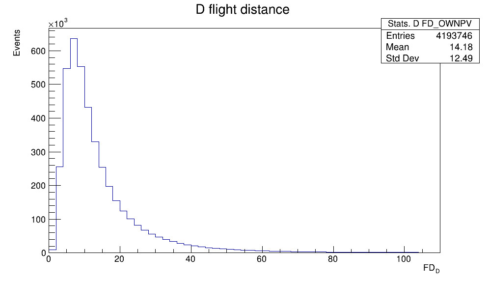
Variables employed for the selection
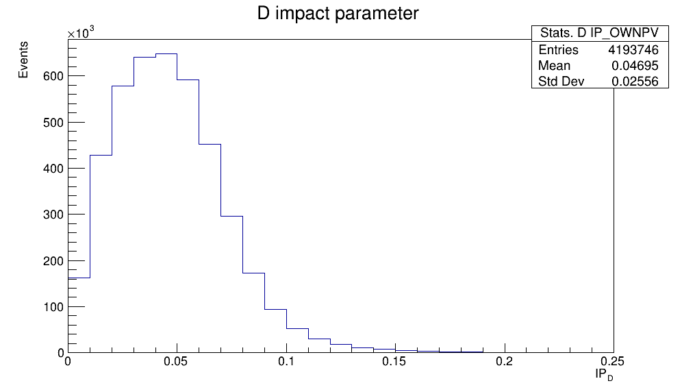
Variables employed for the selection
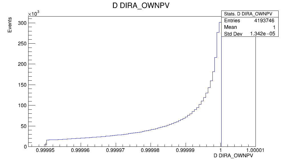
Variables employed for the selection
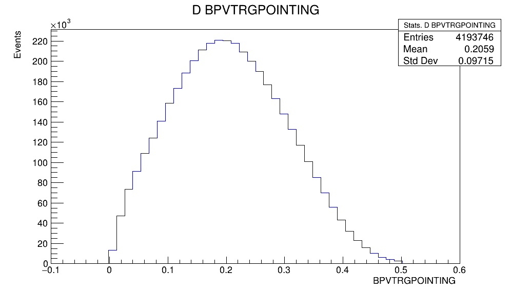
Variables employed for the selection
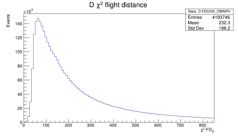
Variables employed for the selection
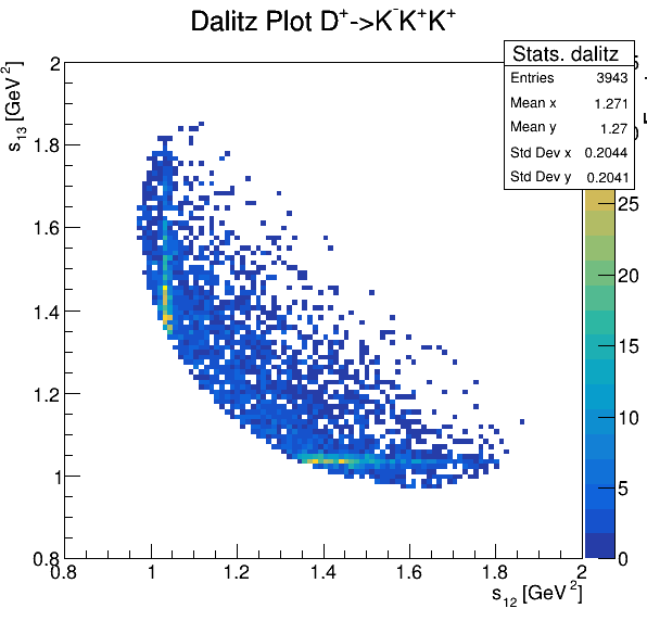
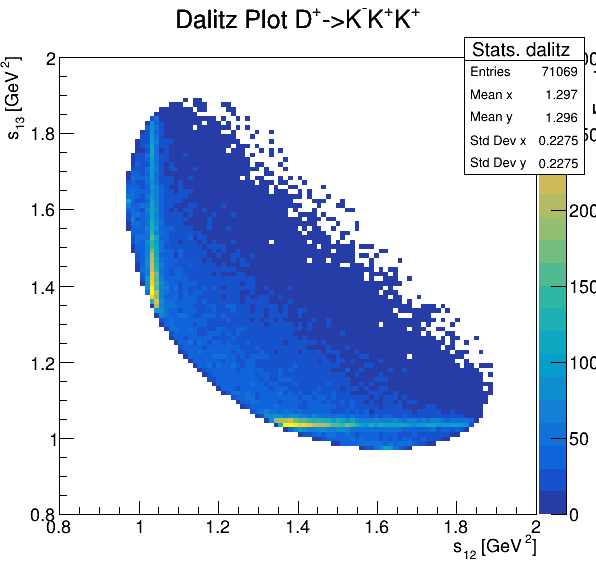
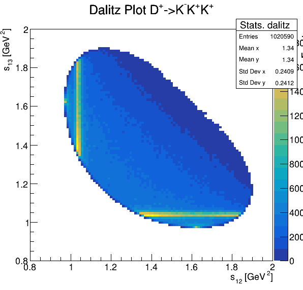
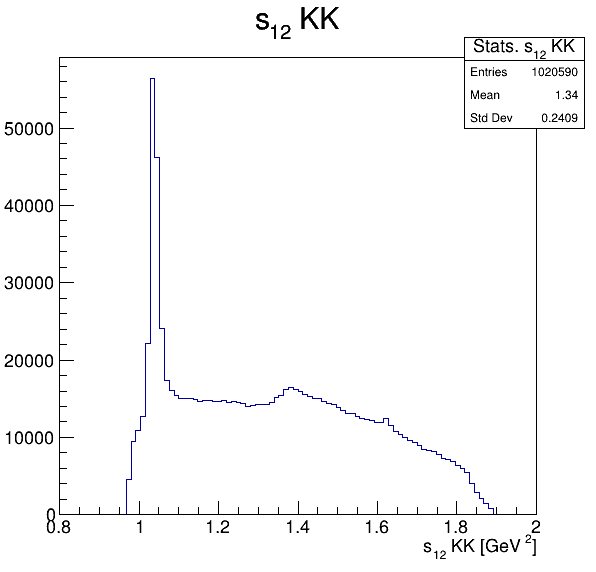
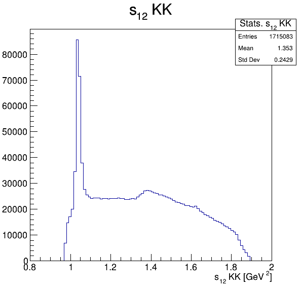
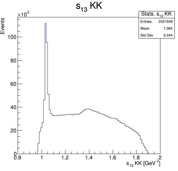
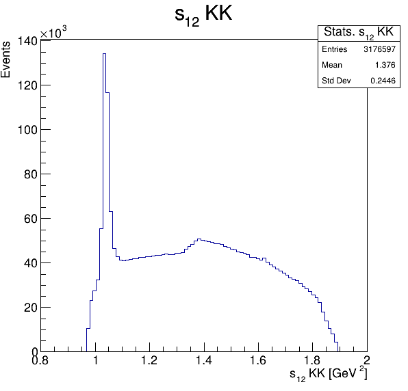
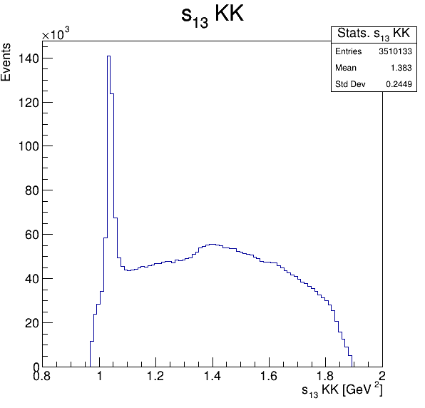
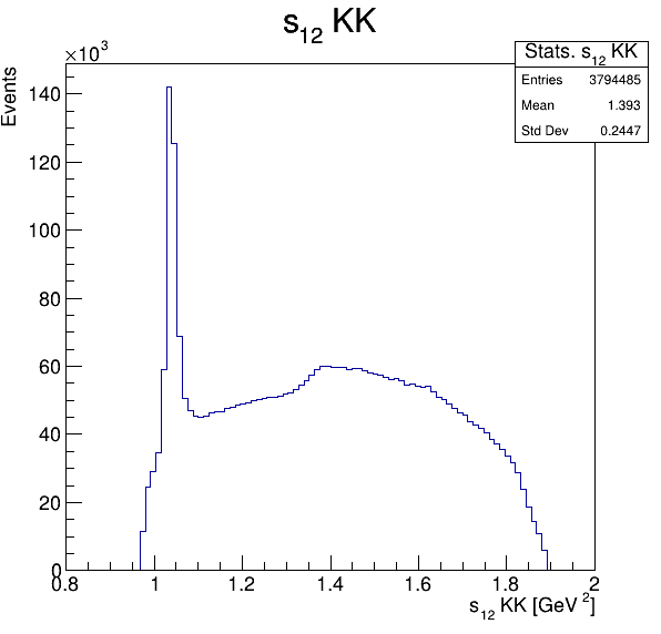
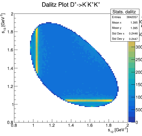
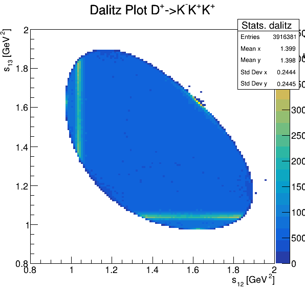
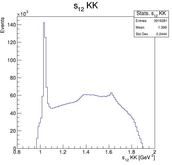
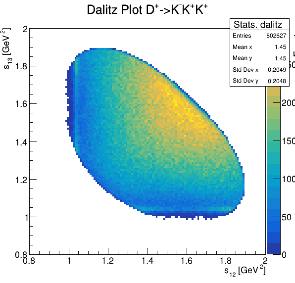
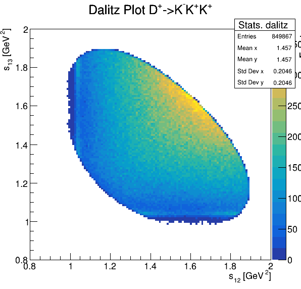
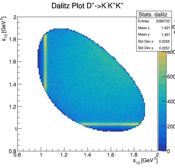
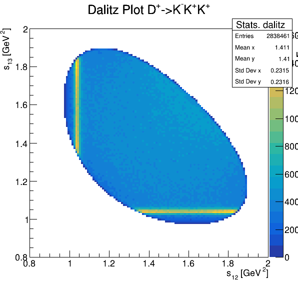
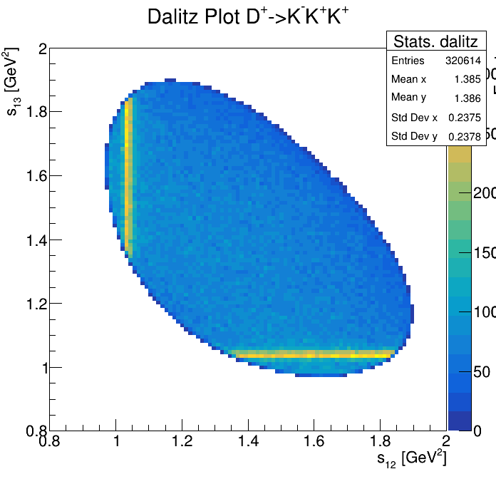
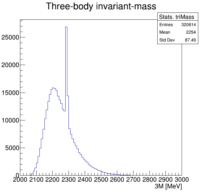
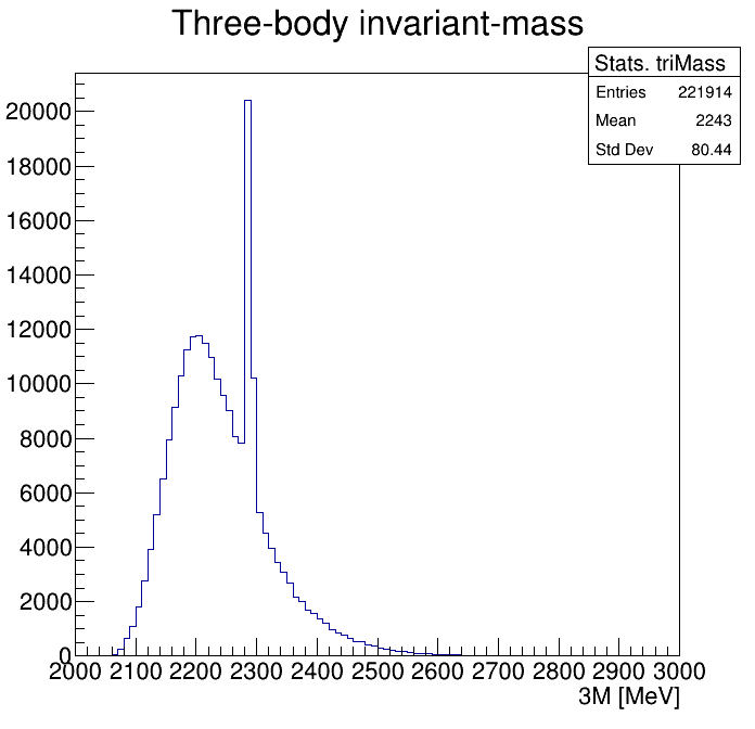
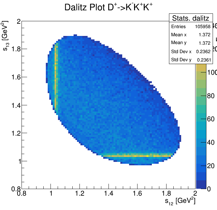
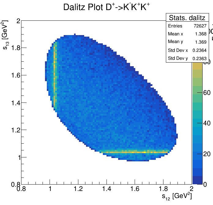
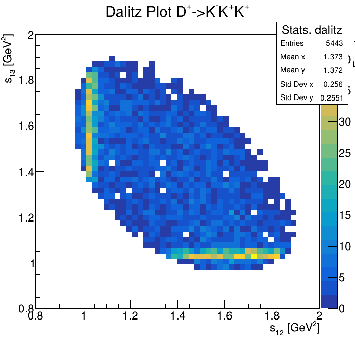
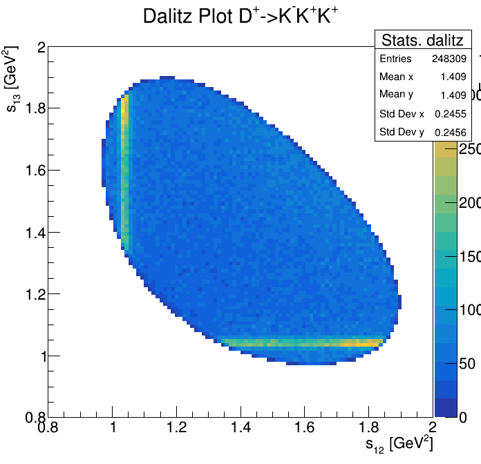
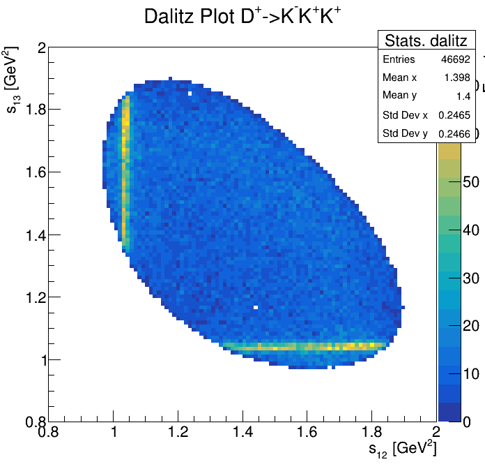
Square of the two-body invariant masses
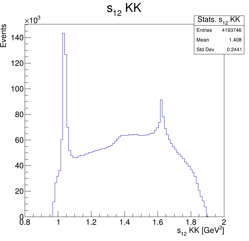
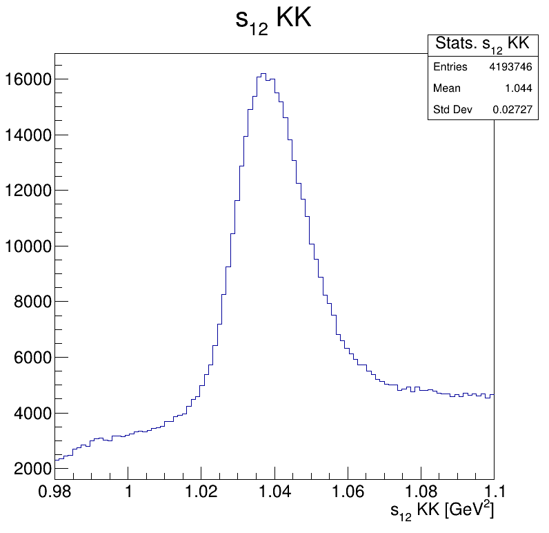
\(\phi(1020)\)
Fake background!
A closer look
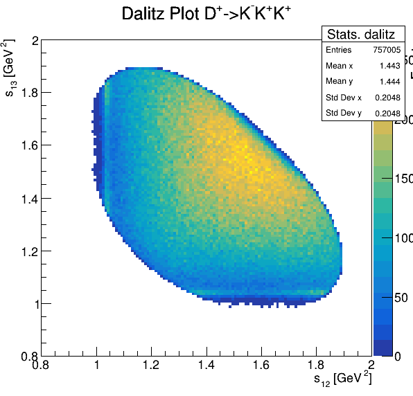
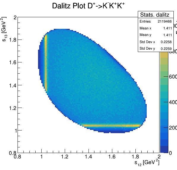
Square of the two-body invariant masses
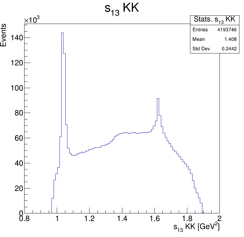

Background!
Zoom
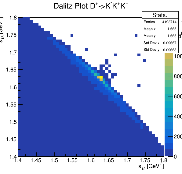
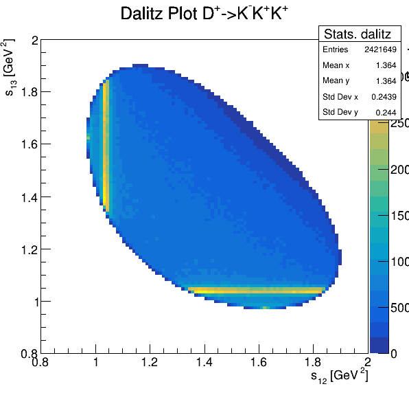
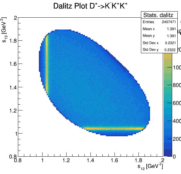
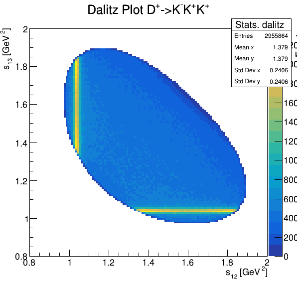
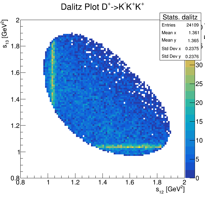
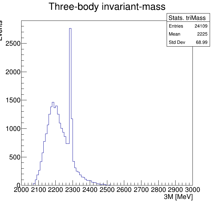
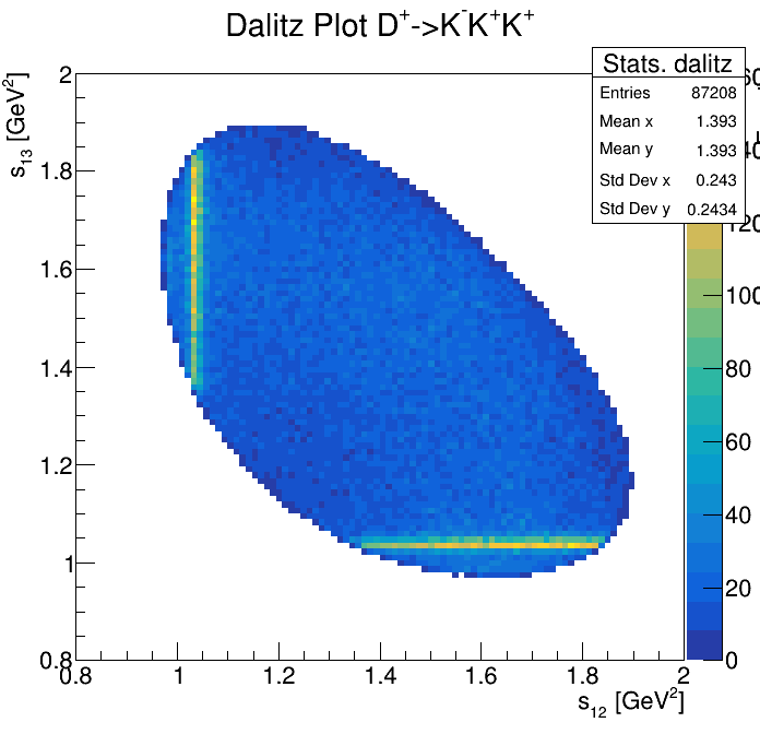
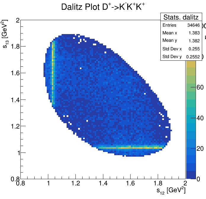
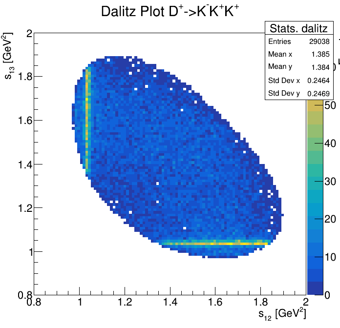
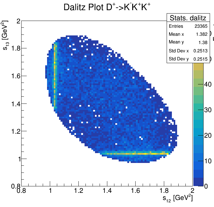
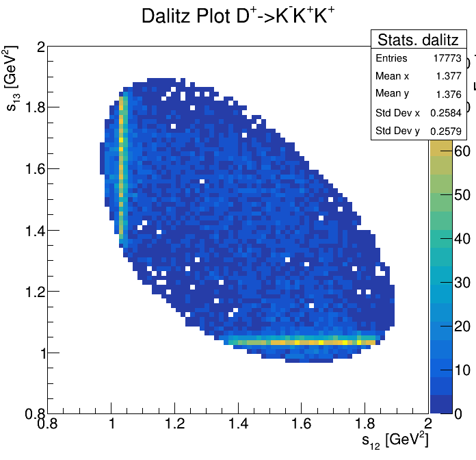
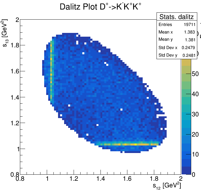
Dalitz plot
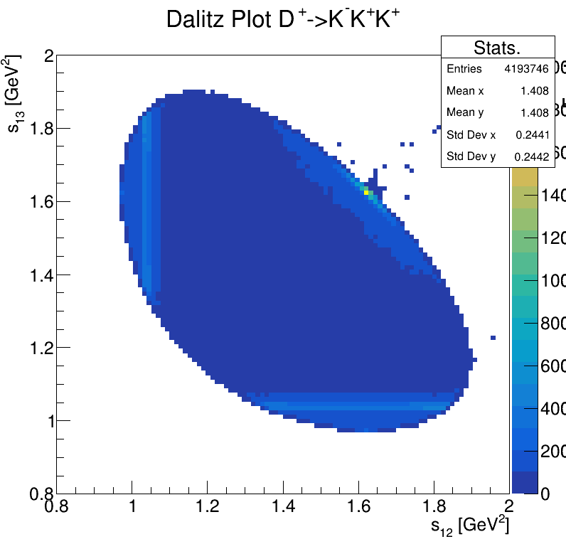
Original data
Fake background
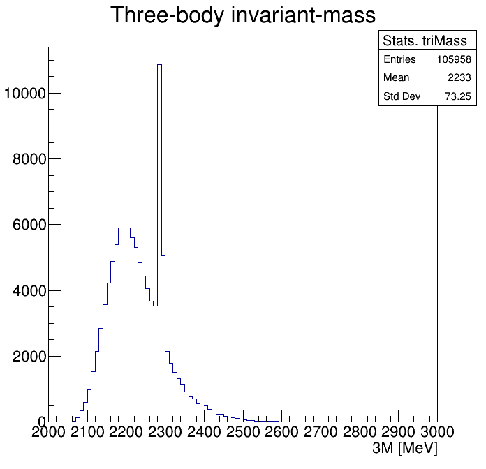
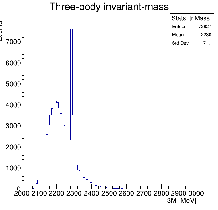
Background coming from the wrong reconstruction of a couple of kaons as just one. This is due to the fact that the angle between the assocciated tracks is quite small and then the identification fails.
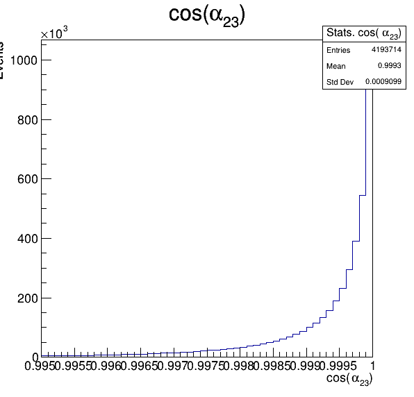
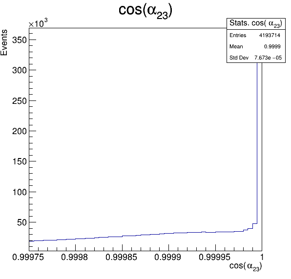
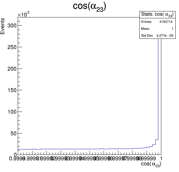
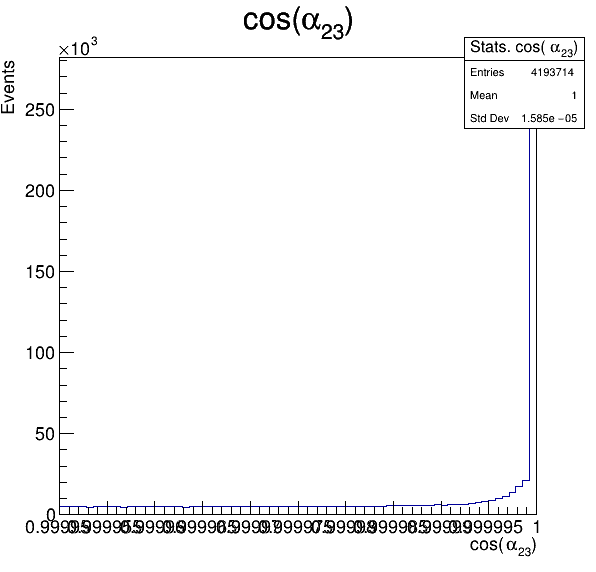
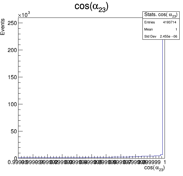
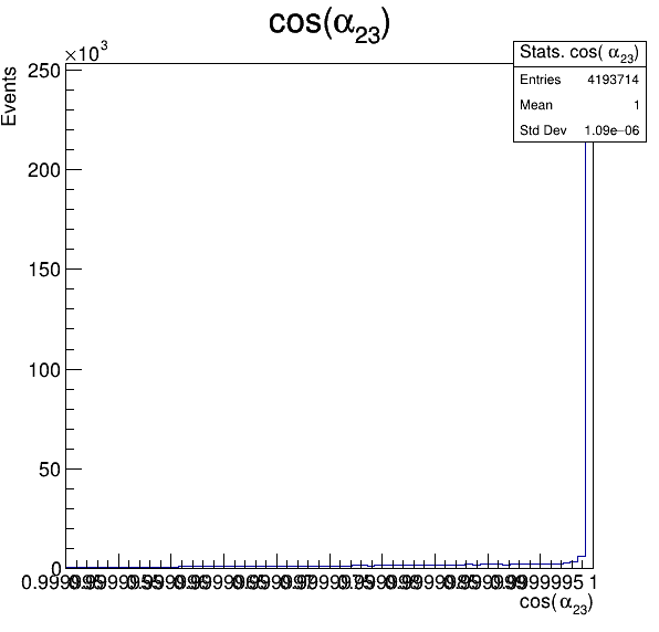
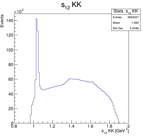
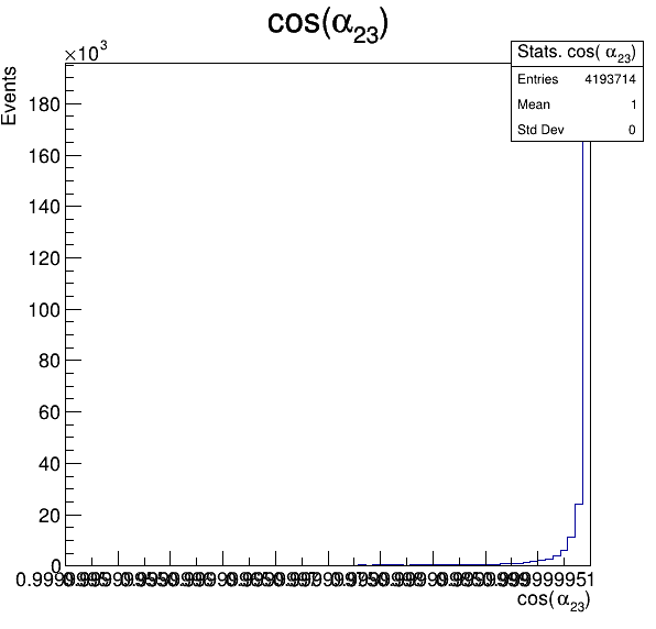
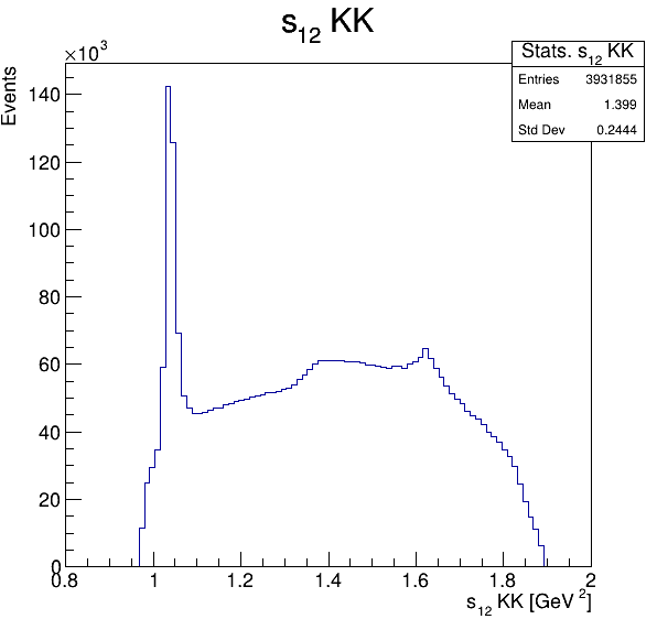
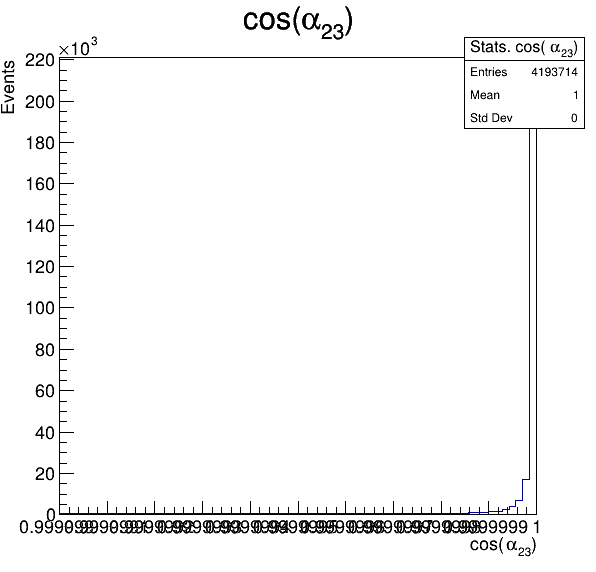
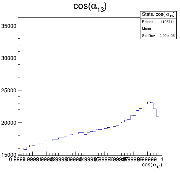
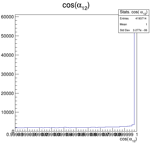
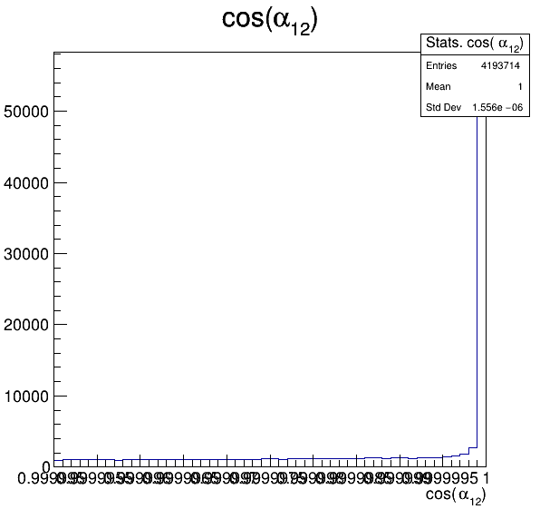
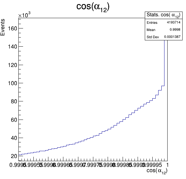
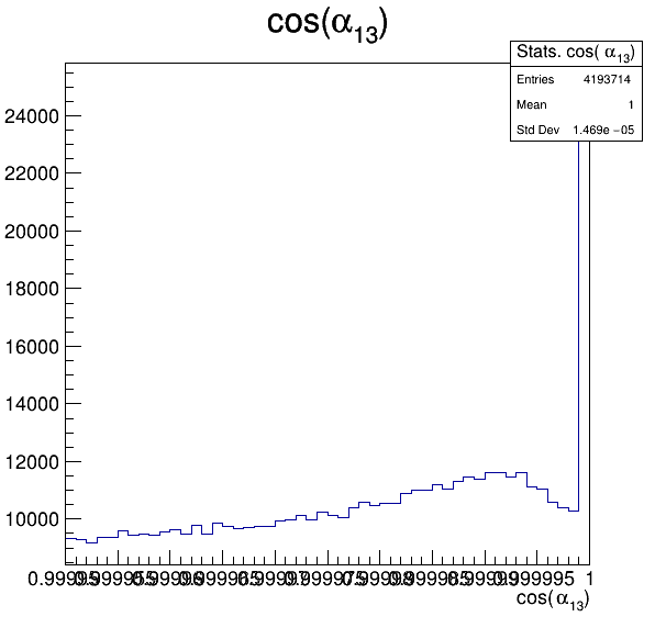
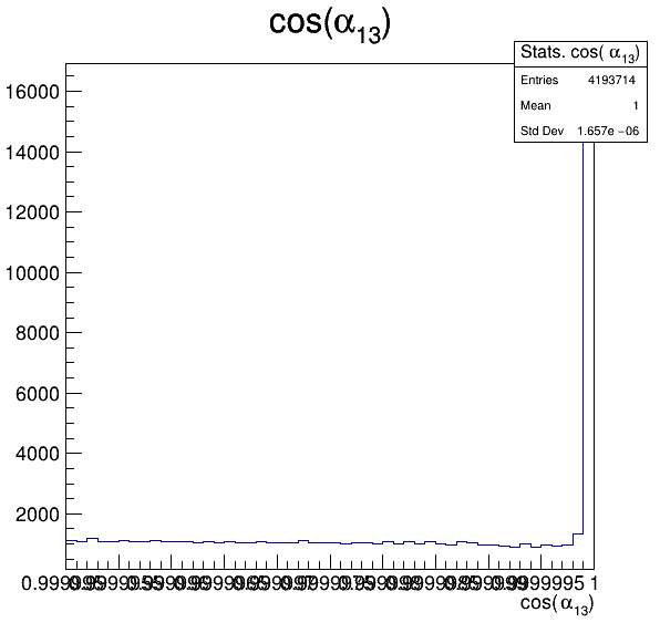
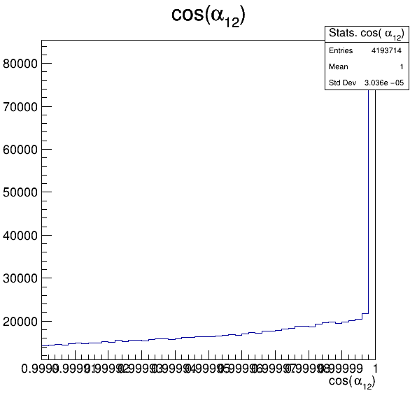
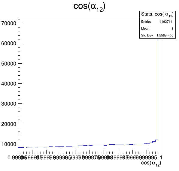
Fake background: \(\cos(\alpha_{K_{2}^{+}K_{3}^{+}})\)
In order to reject fake background it was used the angle between the kaons, i.e.
\boxed{\cos(\alpha_{K_{1}K_{2}})=\frac{p_{1x}p_{2x}+p_{1y}p_{2y}+p_{1z}p_{2z}}{p_{1}p_{2}}}
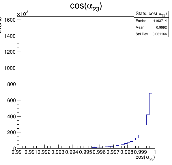
\cos(\alpha_{23})<0.99
Fake background: \(\cos(\alpha_{K_{2}^{+}K_{3}^{+}})\)
\cos(\alpha_{23})<0.995
1.
Fake background: \(\cos(\alpha_{K_{2}^{+}K_{3}^{+}})\)
\cos(\alpha_{23})<0.999
2.
Fake background: \(\cos(\alpha_{K_{2}^{+}K_{3}^{+}})\)
2.

Fake background: \(\cos(\alpha_{K_{2}^{+}K_{3}^{+}})\)
3.
\cos(\alpha_{23})<0.9995

Fake background: \(\cos(\alpha_{K_{2}^{+}K_{3}^{+}})\)
3.

Fake background: \(\cos(\alpha_{K_{2}^{+}K_{3}^{+}})\)
4.
\cos(\alpha_{23})<0.99975
Fake background: \(\cos(\alpha_{K_{2}^{+}K_{3}^{+}})\)
4.

Fake background: \(\cos(\alpha_{K_{2}^{+}K_{3}^{+}})\)
5.
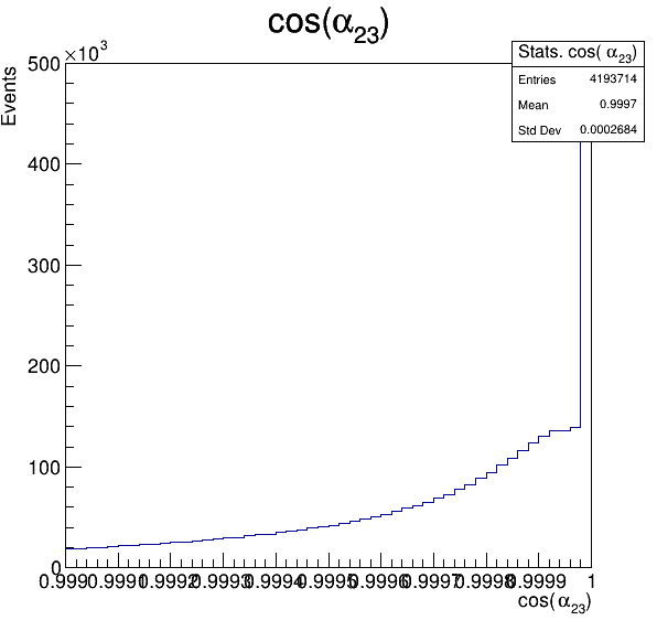
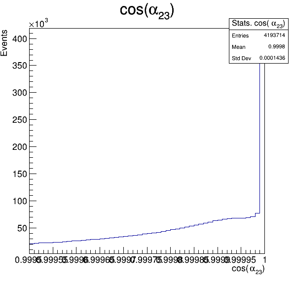
\cos(\alpha_{23})<0.9999

Fake background: \(\cos(\alpha_{K_{2}^{+}K_{3}^{+}})\)
5.

Fake background: \(\cos(\alpha_{K_{2}^{+}K_{3}^{+}})\)
6.
\cos(\alpha_{23})<0.99995

Fake background: \(\cos(\alpha_{K_{2}^{+}K_{3}^{+}})\)
6.

Fake background: \(\cos(\alpha_{K_{2}^{+}K_{3}^{+}})\)
7.
\cos(\alpha_{23})<0.99999

Fake background: \(\cos(\alpha_{K_{2}^{+}K_{3}^{+}})\)
7.

Fake background: \(\cos(\alpha_{K_{2}^{+}K_{3}^{+}})\)
8.
\cos(\alpha_{23})<0.999995
Fake background: \(\cos(\alpha_{K_{2}^{+}K_{3}^{+}})\)
8.

Fake background: \(\cos(\alpha_{K_{2}^{+}K_{3}^{+}})\)
8.
\cos(\alpha_{23})<0.9999995

Fake background: \(\cos(\alpha_{K_{2}^{+}K_{3}^{+}})\)
8.

Fake background: \(\cos(\alpha_{K_{2}^{+}K_{3}^{+}})\)
9.
\cos(\alpha_{23})<0.999999
Fake background: \(\cos(\alpha_{K_{2}^{+}K_{3}^{+}})\)
9.

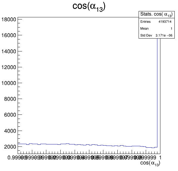
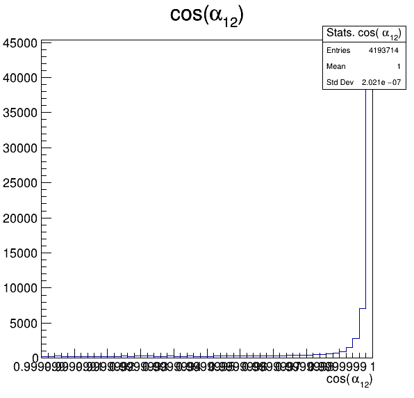
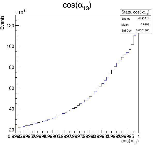
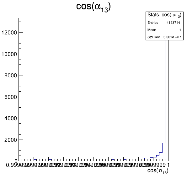
Fake background: \(\cos(\alpha_{K_{1}^{-}K_{2}^{+}})\) and \(\cos(\alpha_{K_{1}^{-}K_{3}^{+}})\)
\boxed{\cos(\alpha_{23})<0.9999}
\cos(\alpha_{12})<0.9995
\cos(\alpha_{13})<0.9995


5.1
Fake background: \(\cos(\alpha_{K_{1}^{-}K_{2}^{+}})\) and \(\cos(\alpha_{K_{1}^{-}K_{3}^{+}})\)
\boxed{\cos(\alpha_{23})<0.9999}
\cos(\alpha_{12})<0.9999
\cos(\alpha_{13})<0.9999


5.2
Fake background: \(\cos(\alpha_{K_{1}^{-}K_{2}^{+}})\) and \(\cos(\alpha_{K_{1}^{-}K_{3}^{+}})\)
\boxed{\cos(\alpha_{23})<0.9999}
\cos(\alpha_{12})<0.99995
\cos(\alpha_{13})<0.99995


5.3
Fake background: \(\cos(\alpha_{K_{1}^{-}K_{2}^{+}})\) and \(\cos(\alpha_{K_{1}^{-}K_{3}^{+}})\)
\boxed{\cos(\alpha_{23})<0.9999}
\cos(\alpha_{12})<0.99999
\cos(\alpha_{13})<0.99999
5.4
Fake background: \(\cos(\alpha_{K_{1}^{-}K_{2}^{+}})\) and \(\cos(\alpha_{K_{1}^{-}K_{3}^{+}})\)
\boxed{\cos(\alpha_{23})<0.9999}
\cos(\alpha_{12})<0.999995
\cos(\alpha_{13})<0.999995


5.5
Fake background: \(\cos(\alpha_{K_{1}^{-}K_{2}^{+}})\) and \(\cos(\alpha_{K_{1}^{-}K_{3}^{+}})\)
\boxed{\cos(\alpha_{23})<0.9999}
\cos(\alpha_{12})<0.999999
\cos(\alpha_{13})<0.999999


5.6
Fake background: \(\cos(\alpha_{K_{1}^{-}K_{2}^{+}})\) and \(\cos(\alpha_{K_{1}^{-}K_{3}^{+}})\)
\boxed{\cos(\alpha_{23})<0.99995}
\cos(\alpha_{12})<0.9995
\cos(\alpha_{13})<0.9995

6.1
Fake background: \(\cos(\alpha_{K_{1}^{-}K_{2}^{+}})\) and \(\cos(\alpha_{K_{1}^{-}K_{3}^{+}})\)
\boxed{\cos(\alpha_{23})<0.99995}
\cos(\alpha_{12})<0.9999
\cos(\alpha_{13})<0.9999


6.2
Fake background: \(\cos(\alpha_{K_{1}^{-}K_{2}^{+}})\) and \(\cos(\alpha_{K_{1}^{-}K_{3}^{+}})\)
\boxed{\cos(\alpha_{23})<0.99995}
\cos(\alpha_{12})<0.99995
\cos(\alpha_{13})<0.99995


6.3
Fake background: \(\cos(\alpha_{K_{1}^{-}K_{2}^{+}})\) and \(\cos(\alpha_{K_{1}^{-}K_{3}^{+}})\)
\boxed{\cos(\alpha_{23})<0.99995}
\cos(\alpha_{12})<0.99999
\cos(\alpha_{13})<0.99999


6.4
Fake background: \(\cos(\alpha_{K_{1}^{-}K_{2}^{+}})\) and \(\cos(\alpha_{K_{1}^{-}K_{3}^{+}})\)
\boxed{\cos(\alpha_{23})<0.99995}
\cos(\alpha_{12})<0.999995
\cos(\alpha_{13})<0.999995


6.5
Fake background: \(\cos(\alpha_{K_{1}^{-}K_{2}^{+}})\) and \(\cos(\alpha_{K_{1}^{-}K_{3}^{+}})\)
\boxed{\cos(\alpha_{23})<0.99995}
\cos(\alpha_{12})<0.999999
\cos(\alpha_{13})<0.999999


6.6
Fake background: \(\cos(\alpha_{K_{1}^{-}K_{2}^{+}})\) and \(\cos(\alpha_{K_{1}^{-}K_{3}^{+}})\)
\boxed{\cos(\alpha_{23})<0.99999}
\cos(\alpha_{12})<0.9995
\cos(\alpha_{13})<0.9995

7.1
Fake background: \(\cos(\alpha_{K_{1}^{-}K_{2}^{+}})\) and \(\cos(\alpha_{K_{1}^{-}K_{3}^{+}})\)
\boxed{\cos(\alpha_{23})<0.99999}
\cos(\alpha_{12})<0.9999
\cos(\alpha_{13})<0.9999

7.2
Fake background: \(\cos(\alpha_{K_{1}^{-}K_{2}^{+}})\) and \(\cos(\alpha_{K_{1}^{-}K_{3}^{+}})\)
\boxed{\cos(\alpha_{23})<0.99999}
\cos(\alpha_{12})<0.99995
\cos(\alpha_{13})<0.99995

7.3
Fake background: \(\cos(\alpha_{K_{1}^{-}K_{2}^{+}})\) and \(\cos(\alpha_{K_{1}^{-}K_{3}^{+}})\)
\boxed{\cos(\alpha_{23})<0.99999}
\cos(\alpha_{12})<0.99999
\cos(\alpha_{13})<0.99999


7.4
Fake background: \(\cos(\alpha_{K_{1}^{-}K_{2}^{+}})\) and \(\cos(\alpha_{K_{1}^{-}K_{3}^{+}})\)
\boxed{\cos(\alpha_{23})<0.99999}
\cos(\alpha_{12})<0.999995
\cos(\alpha_{13})<0.999995


7.5
Fake background: \(\cos(\alpha_{K_{1}^{-}K_{2}^{+}})\) and \(\cos(\alpha_{K_{1}^{-}K_{3}^{+}})\)
\boxed{\cos(\alpha_{23})<0.99999}
\cos(\alpha_{12})<0.999999
\cos(\alpha_{13})<0.999999


7.6
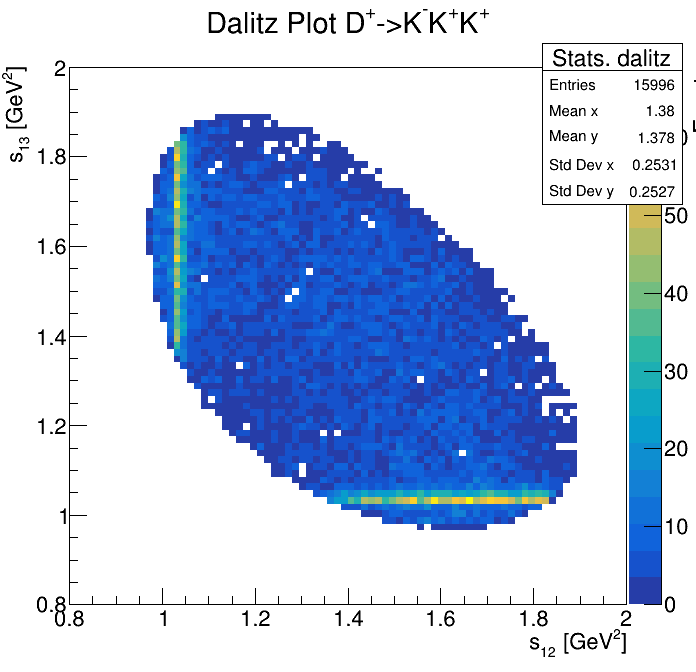
Fake background: Possible best cuts
5.4
5.5
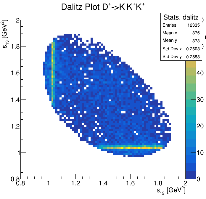
Fake background: Possible best cuts
6.5
6.4
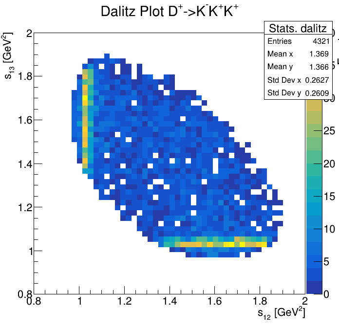
Fake background: Possible best cuts
7.5
7.4
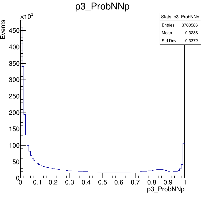
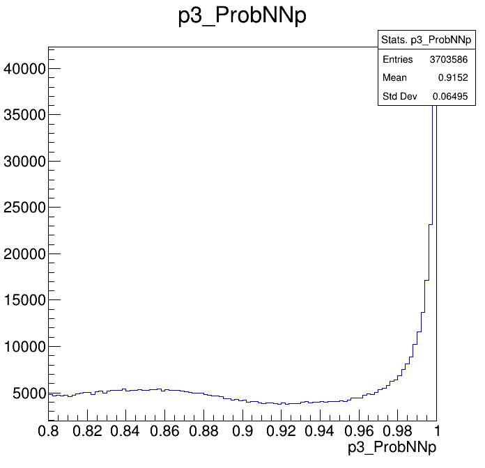
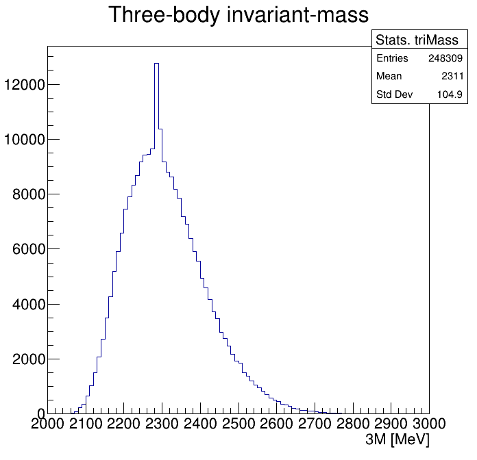
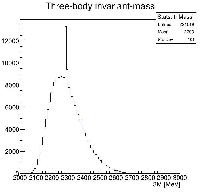
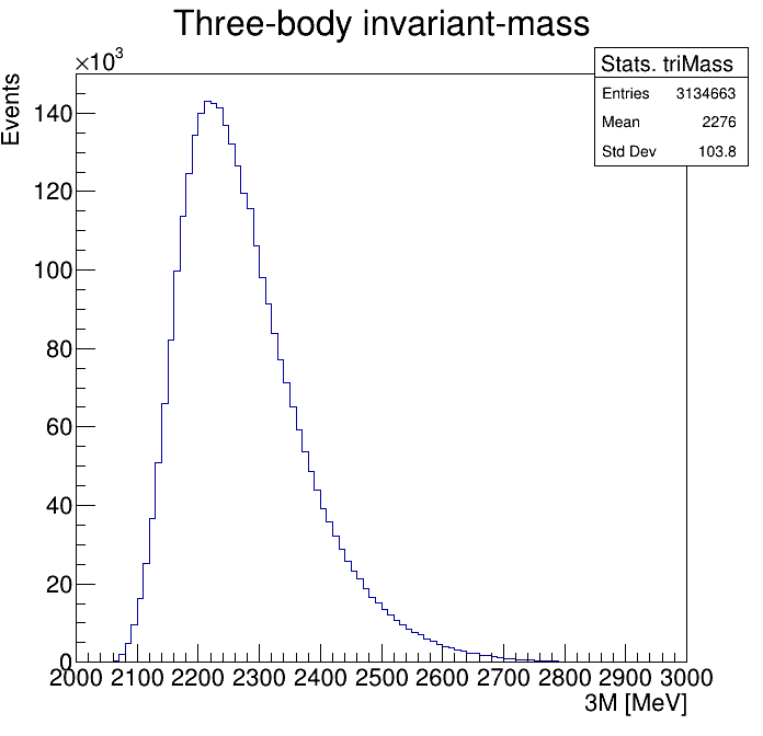
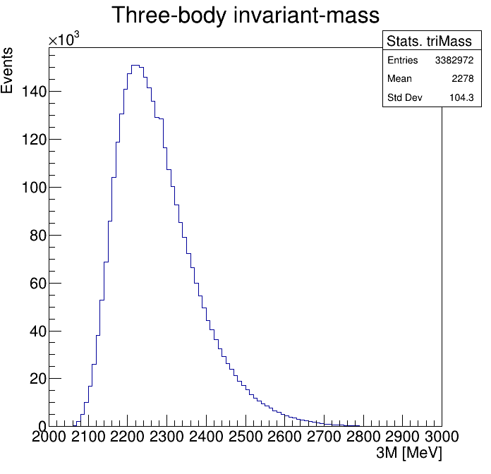
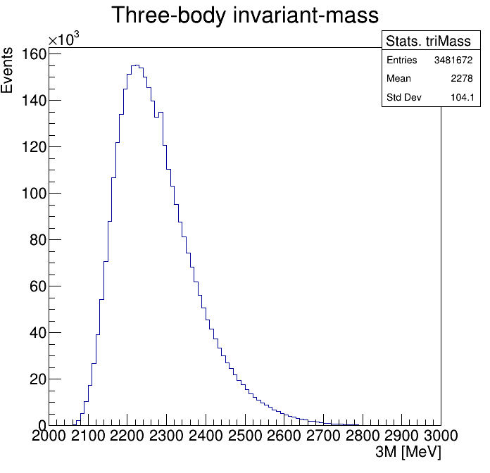
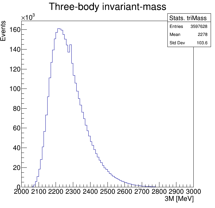
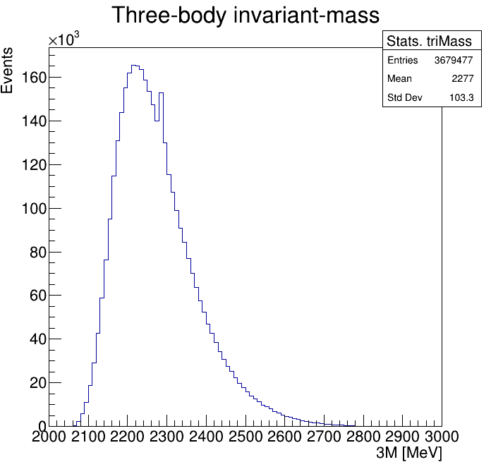
Physical Background: \(\Lambda^{+}_{c}\longrightarrow K^{-}K^{+}p\)
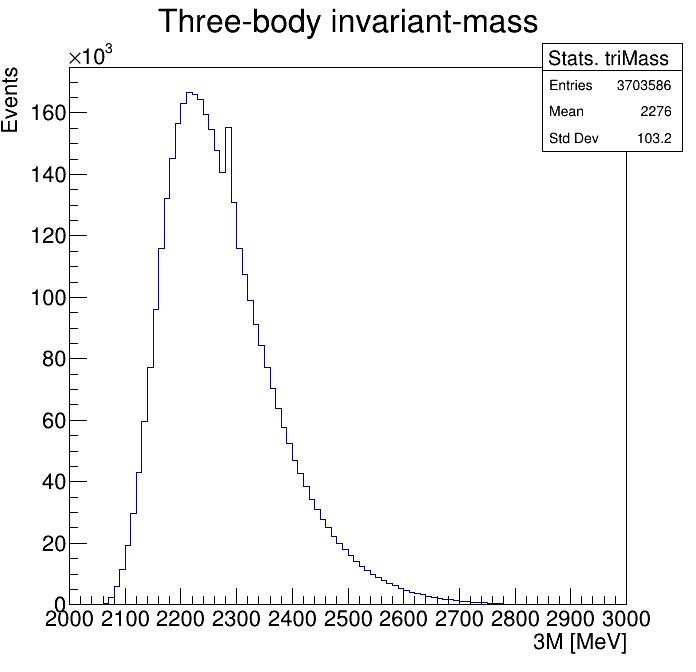
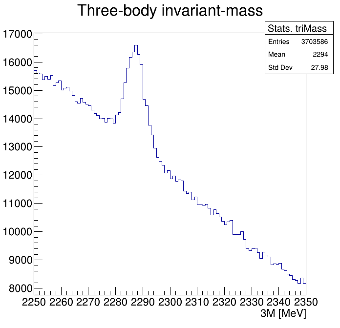
Physical Background: \(\Lambda^{+}_{c}\longrightarrow K^{-}K^{+}p\)
Physical Background: \(\Lambda^{+}_{c}\longrightarrow K^{-}K^{+}p\)
p3_ProbNNp>0.9
Physical Background: \(\Lambda^{+}_{c}\longrightarrow K^{-}K^{+}p\)
p3_ProbNNp>0.95

Physical Background: \(\Lambda^{+}_{c}\longrightarrow K^{-}K^{+}p\)
p3_ProbNNp>0.99
Physical Background: \(\Lambda^{+}_{c}\longrightarrow K^{-}K^{+}p\)
p3_ProbNNp>0.995
Physical Background: \(\Lambda^{+}_{c}\longrightarrow K^{-}K^{+}p\)
p3_ProbNNp>0.999
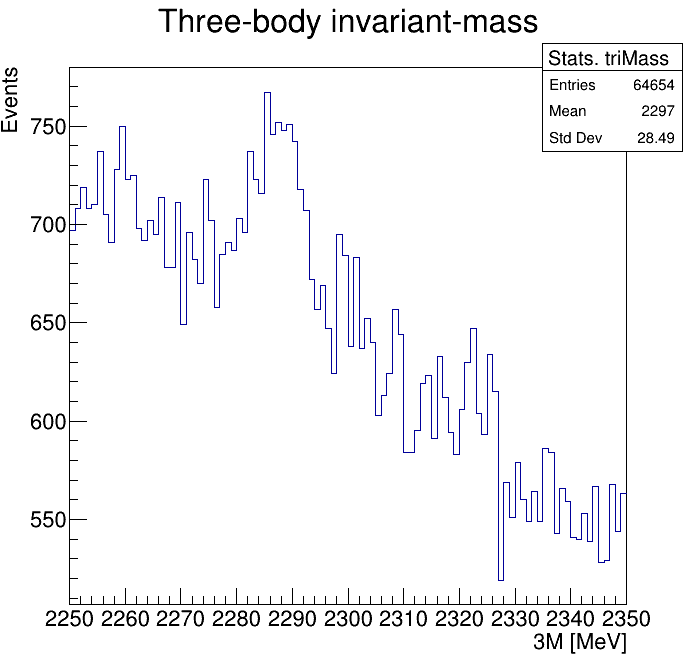
Physical Background: \(\Lambda^{+}_{c}\longrightarrow K^{-}K^{+}p\)
2255\(<m_{KKp}<\)2320
p3_ProbNNp>0.9
2265\(<m_{KKp}<\)2310
2275\(<m_{KKp}<\)2300


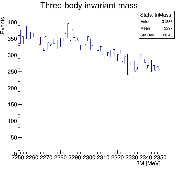
Physical Background: \(\Lambda^{+}_{c}\longrightarrow K^{-}K^{+}p\)
p3_ProbNNp>0.95
2265\(<m_{KKp}<\)2310
2275\(<m_{KKp}<\)2300
2255\(<m_{KKp}<\)2320


Physical Background: \(\Lambda^{+}_{c}\longrightarrow K^{-}K^{+}p\)
p3_ProbNNp>0.99
2265\(<m_{KKp}<\)2310
2275\(<m_{KKp}<\)2300
2255\(<m_{KKp}<\)2320
Physical Background: \(\Lambda^{+}_{c}\longrightarrow K^{-}K^{+}p\)
p3_ProbNNp>0.995
2265\(<m_{KKp}<\)2310
2275\(<m_{KKp}<\)2300
2255\(<m_{KKp}<\)2320
Physical Background: \(\Lambda^{+}_{c}\longrightarrow K^{-}K^{+}p\)
p3_ProbNNp>0.999
2265\(<m_{KKp}<\)2310
2275\(<m_{KKp}<\)2300
2255\(<m_{KKp}<\)2320

Physical Background: \(\Lambda^{+}_{c}\longrightarrow K^{-}K^{+}p\)
0.8<p3_ProbNNp<0.9
Physical Background: \(\Lambda^{+}_{c}\longrightarrow K^{-}K^{+}p\)
0.8<p3_ProbNNp<0.9
2255\(<m_{KKp}<\)2320
2265\(<m_{KKp}<\)2310
2275\(<m_{KKp}<\)2300


Physical Background: \(\Lambda^{+}_{c}\longrightarrow K^{-}K^{+}p\)
0.85<p3_ProbNNp<0.95

Physical Background: \(\Lambda^{+}_{c}\longrightarrow K^{-}K^{+}p\)
0.85<p3_ProbNNp<0.95
2265\(<m_{KKp}<\)2310

2255\(<m_{KKp}<\)2320
2275\(<m_{KKp}<\)2300


Physical Background: \(\Lambda^{+}_{c}\longrightarrow K^{-}K^{+}p\)
p3_ProbNNp<0.8

Physical Background: \(\Lambda^{+}_{c}\longrightarrow K^{-}K^{+}p\)
p3_ProbNNp<0.9

Physical Background: \(\Lambda^{+}_{c}\longrightarrow K^{-}K^{+}p\)
p3_ProbNNp<0.95

Physical Background: \(\Lambda^{+}_{c}\longrightarrow K^{-}K^{+}p\)
p3_ProbNNp<0.99

Physical Background: \(\Lambda^{+}_{c}\longrightarrow K^{-}K^{+}p\)
p3_ProbNNp<0.995


Physical Background: \(\Lambda^{+}_{c}\longrightarrow K^{-}K^{+}p\)
p3_ProbNNp<0.999

Physical Background: \(\Lambda^{+}_{c}\longrightarrow K^{-}K^{+}p\)
0.6<p3_ProbNNp<0.7
0.6<p3_ProbNNp<0.65
[CERN Summer Programme] Quick presentation 09.07
By Sebastian Ordoñez


