Sebastián Ordoñez-Soto
Universidad Nacional de Colombia
Internship tutor: Patrick Robbe
Guidance: Liupan An
July 7th, 2023


Study of VELO-ECAL timing for U1b using the Hybrid-MC toolkit
Internship update-IJCLab LHCb group meeting


Outline
- Introduction
- LHCb VELO and ECAL
- ECAL upgrade scenarios
- Motivation
- Simulation
- Hybrid-MC toolkit
- Workflow
- Results
- Truth level
- Full ECAL simulation
- Reco level
- Summary
Introduction
-
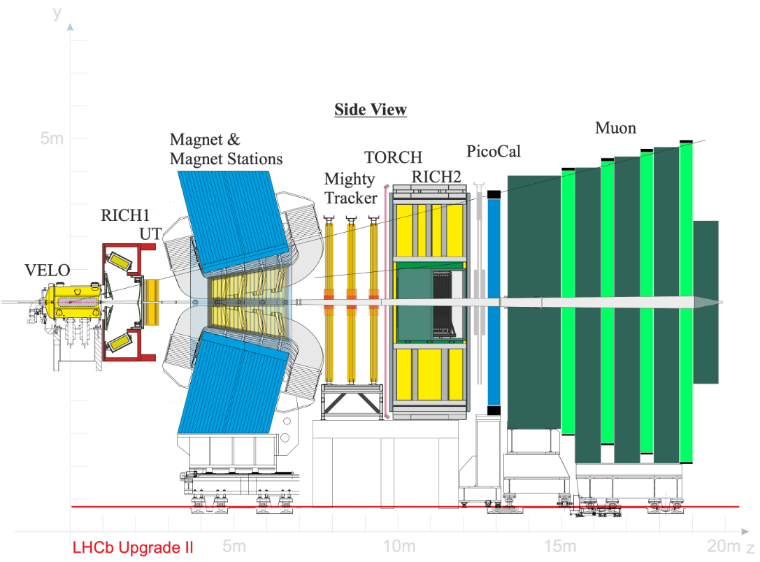
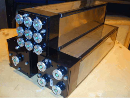
LHCb Electromagnetic CALorimeter (ECAL)
- Designed to measure and identify electromagnetic particles, such as photons and electrons.
- Main purposes: energy measurement, particle identification and precision timing.
-
LHCb VErtex LOcator (VELO)
- Provides measurements of track coordinates close to the interaction region.
- Main purposes: reconstruct production and decay vertices of \(b\) and \(c\) hadrons.
Introduction
-
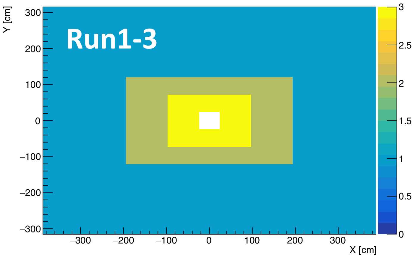
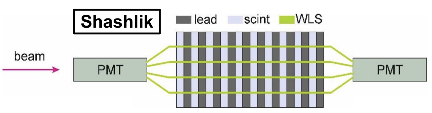
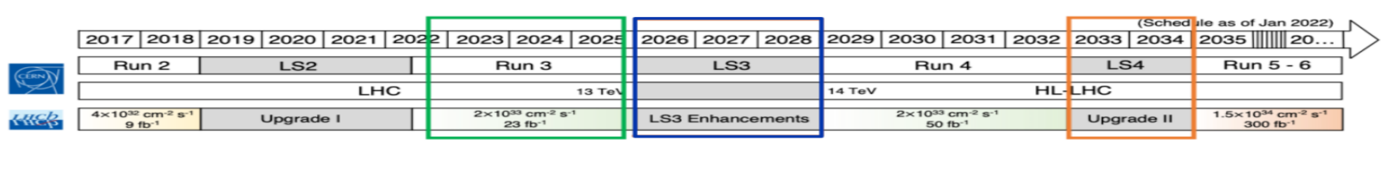
Run 1-3
- Shashlik cells \(4\times4\), \(6\times6\) and \(12\times12\) cm\(^{2}\)
-
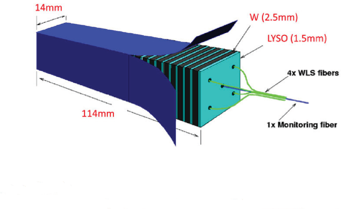
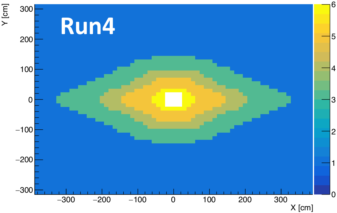
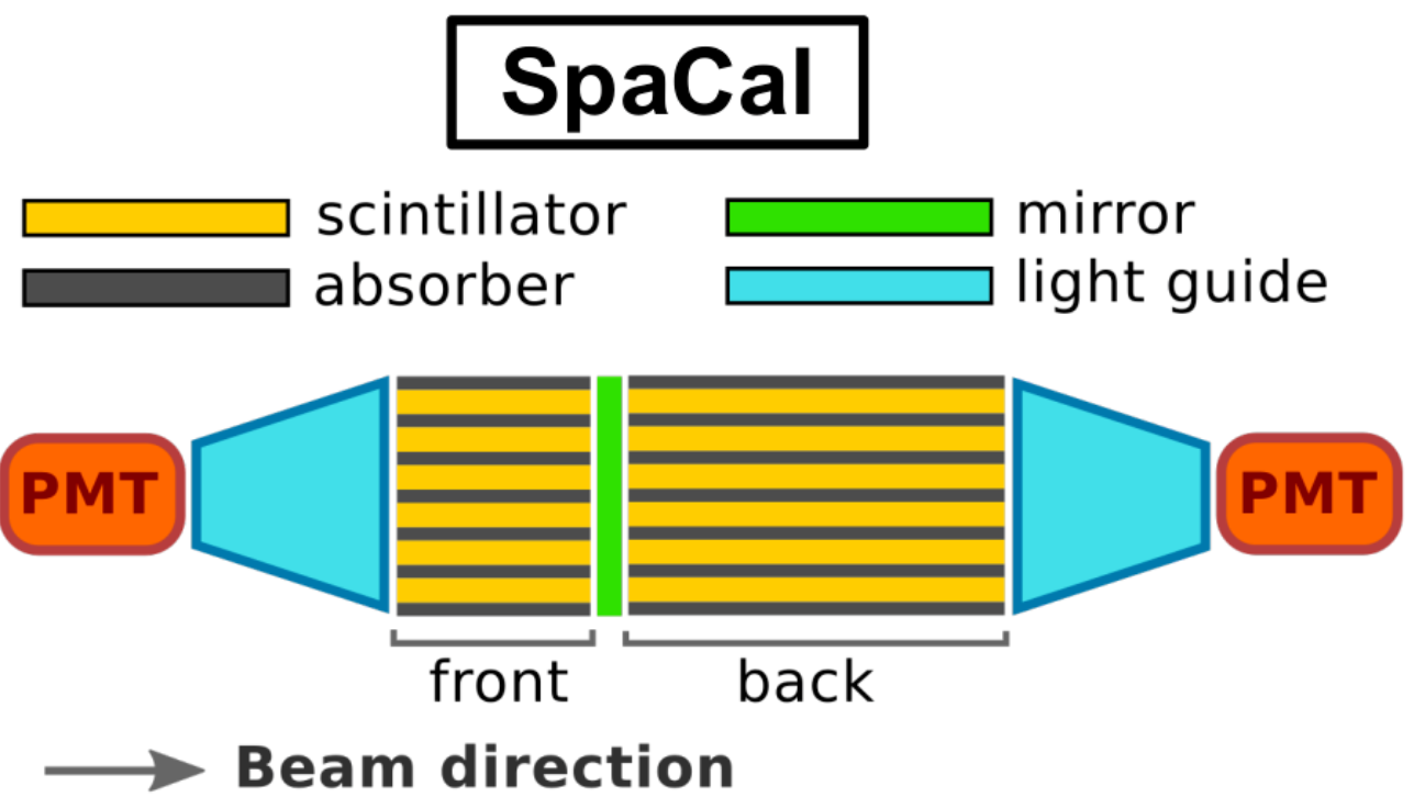
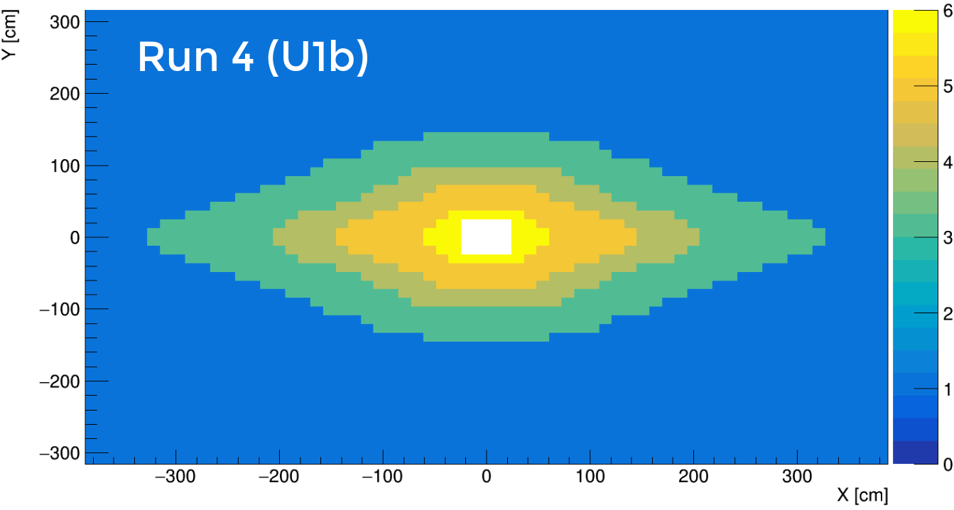
Upgrade 1b (Run 4)
- Innermost: SPACAL W+Poly \(2\times2\) cm\(^{2}\)
- Second inner: SPACAL Pb+Poly \(3\times3\) cm\(^{2}\)
- Outer: Shashlik \(4\times4\), \(6\times6\) and \(12\times12\) cm\(^{2}\)
- No longiudinal segmentation
- Timing readout for SPACAL
-
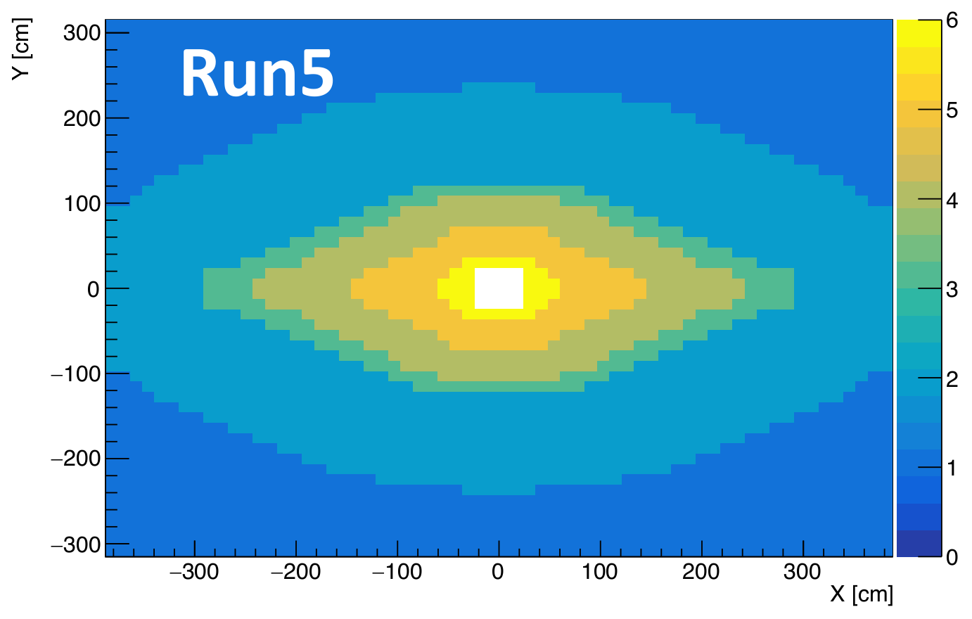
Upgrade 2 (Run 5)
- Innermost: SPACAL W+GAGG \(1.5\times1.5\) cm\(^{2}\)
- Second inner and outer same as for Run 4.
- Longitudinal segmentation
- Dual timing readout for all modules
Introduction
-
This project
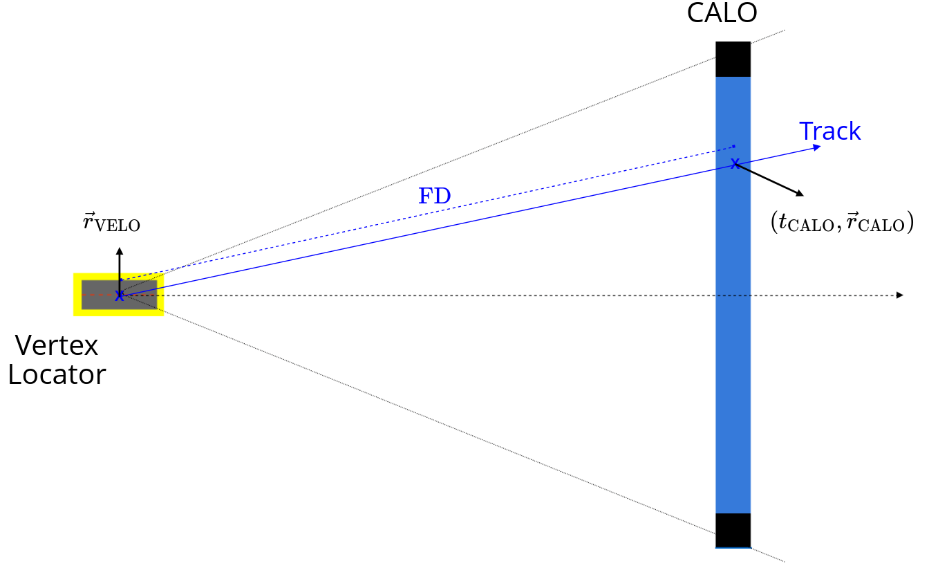
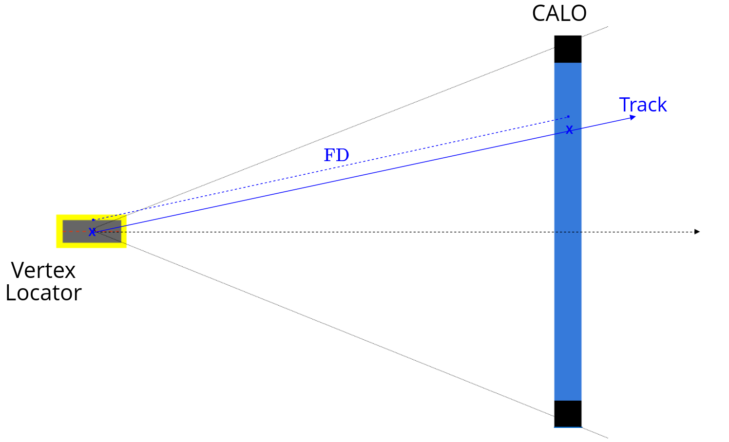
- Analyze the feasibility of estimating U1b VELO timing from VELO/CALO track positions and CALO timing using the Hybrid-MC toolkit.
\boxed{t_{\text{VELO}} \approx t_{\text{CALO}} - \frac{\text{FD}}{\text{V}}}
\boxed{\text{Adding timing will be key to remove a lot of expected pile-up!}}
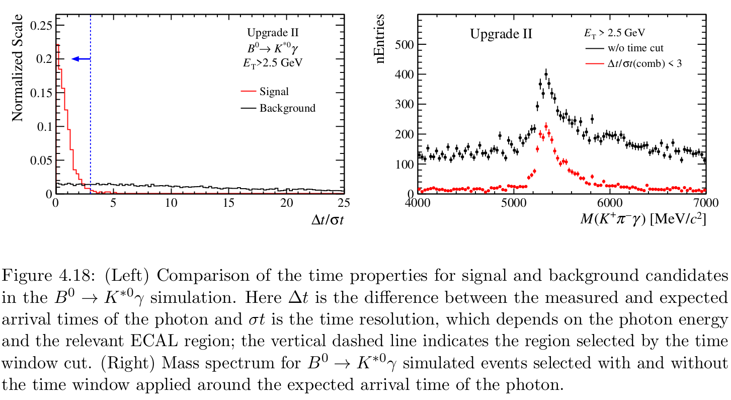
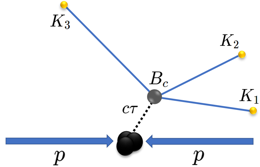
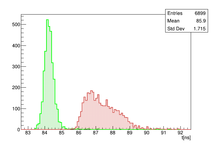
\(B^{0}\rightarrow K^{*0}\gamma \rightarrow (K^{\pm}\pi^{\mp})\gamma\)
Comparison of the time properties for signal and background candidates in the \(B^{0}\rightarrow K^{*0}\gamma\) decay using Upgrade II simulation.
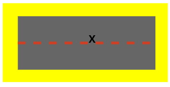
X

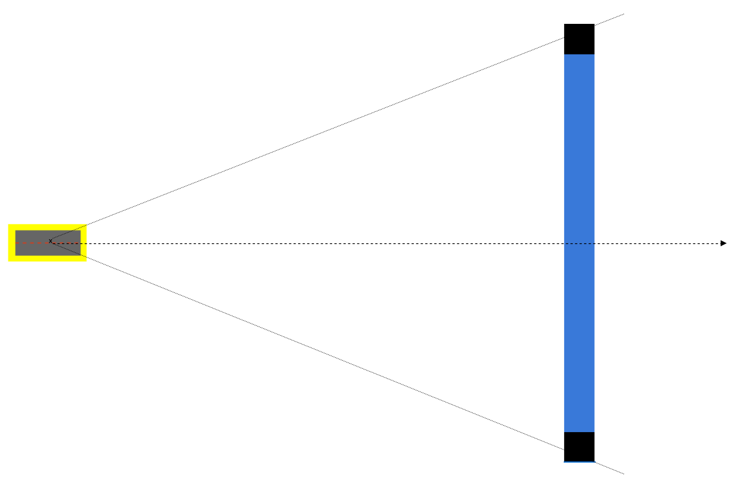
CALO
Vertex
Locator
\boxed{\Delta t = t_{\text{CALO}} - t_{\text{VELO}}}
X
X
Track
\text{FD}
t_{\text{VELO}} \approx t_{\text{CALO}} - \frac{\text{FD}}{\text{V}}
\text{FD} = \vec{r}_{CALO} - \vec{r}_{VELO}
(t_{\text{CALO}},\vec{r}_{\text{CALO}})
(t_{\text{VELO}},\vec{r}_{\text{VELO}})
Simulation
-
Hybrid-MC toolkit
- Geant4 simulation of energy deposit and parametrized transport of scintillation photons
- Perform full-ECAL simulations for Run3 (U1), Run4 (U1b) and Run5 (U2)
- https://gitlab.cern.ch/spacal-rd/spacal-simulation
- Workflow
- Official LHCb MC sample is used as input
Gauss_kstargamma_full_*.sim
- Generate the
flux.root - VELO reconstruction done by VELO team
-
B2Kstgamma_VELO_reco.rootfile
-
- Select events with \(K^{\pm}\pi^{\mp}\) from a \(B^{0}\)
Kpi_tree.root
- Keep only events with Kpi reconstructed
-
match_flux.root
-
Generate flux files
Full ECAL simulation
Reconstruction
- Main config file
- Global characteristics of the ECAL
- Module config files
- Standard configuration files of SPACAL and Shashlik modules
- Map of module types and positions
- CAD drawing of the region(s)
Output: OutTrigd_*.root
- Reads OutTrigd files and gives the final ntuple with cluster reconstructed variables.
Reconstructed_*.root
- Combine with Kpi_tree.root
-
Reconstructed_combined_*.root
-
Results
-
Truth level
-
Flux files
- It is possible to take a look at the timing of tracks which hit the ECAL from the
*.simGauss files
- It is possible to take a look at the timing of tracks which hit the ECAL from the
-
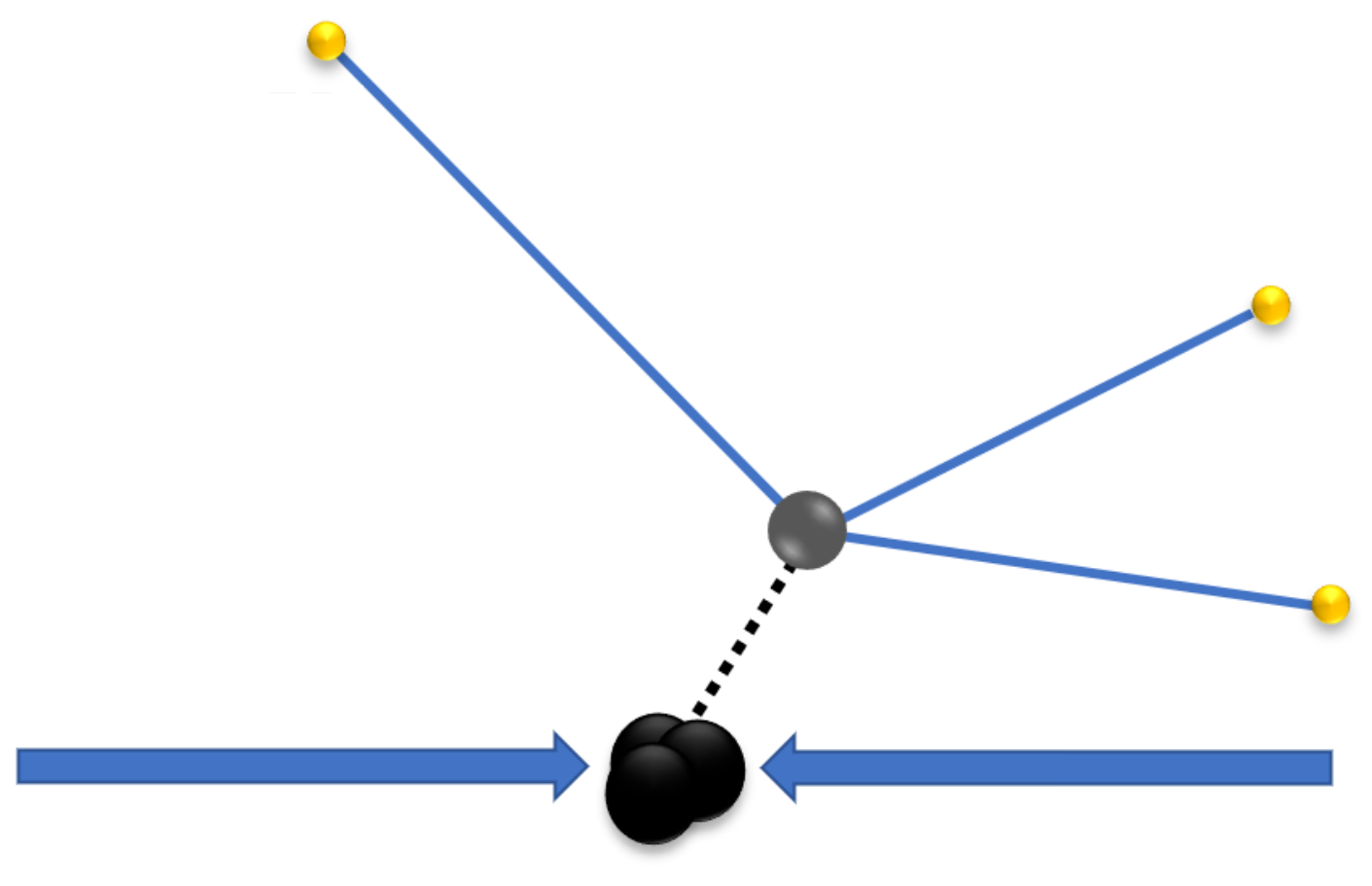
Flux files
p
p
\gamma
K^{\pm}
\pi^{\mp}
B^{0}
-
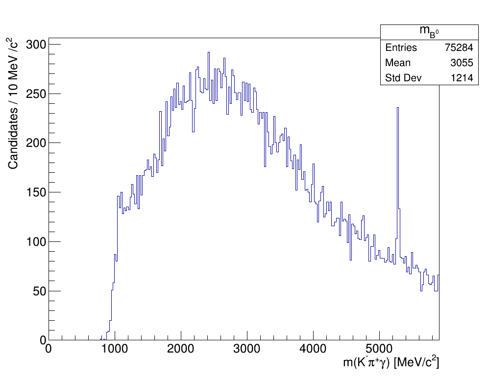
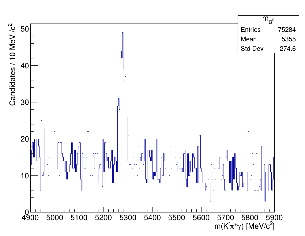
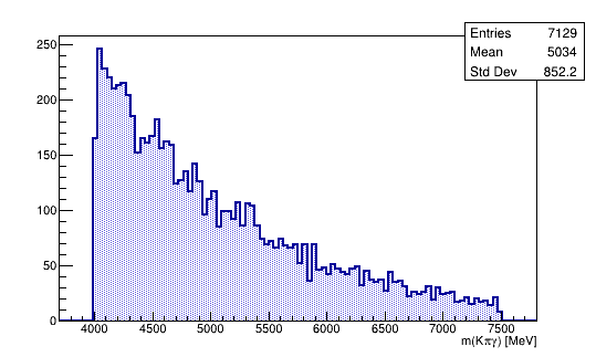
Velo reconstruction
- It is possible to reconstruct the \(B^{0}\) mass spectrum
- Only kaons and pions from a \(B^{0}\) are considered
- As expected, the samples have high levels of background
- It is possible to reconstruct the \(B^{0}\) mass spectrum
Results
-
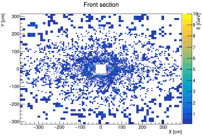
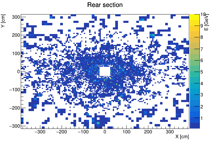
Full ECAL simulation output
- Output of the jobs are
OutTrigd_*.rootfiles, which contains:- ID of the modules hit during the event
- Total number of optical photons detected in the whole calorimeter.
- Number of photons detected in the i-nth cell of the #-nth module in the given event.
- It is possible to obtain the energy deposition from the photon yield in each module for a given configuration.
- Output of the jobs are

Evt: 1evt w/ nPV = 40. Sim: Run 5 config.
Results
-
Reconstruction
- At this point we have the timing (\(t_{K\pi}\)) and position (\(r_{K\pi}\)) of the \(K\pi\) vertex, which are the origin timing and position of the photon.
- We can calculate the flight time from the origin to the ECAL: \(t_{f}\)
- The expected time of the photon to enter ECAL: \(t_{exp} = t_{K\pi}+t_{f}\)
- As result of the simulation we obtain the measured time of the photon cluster: \(t_{obs}\)
- At this point we have the timing (\(t_{K\pi}\)) and position (\(r_{K\pi}\)) of the \(K\pi\) vertex, which are the origin timing and position of the photon.
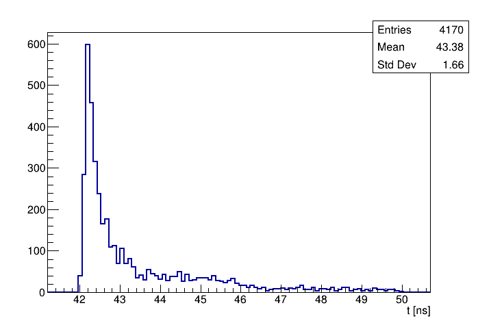
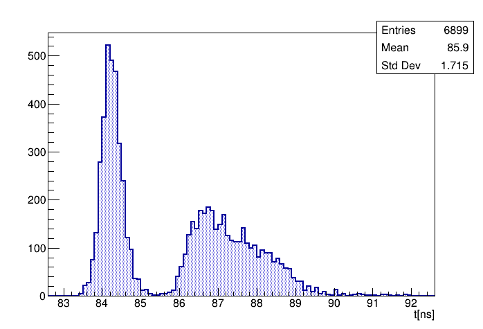
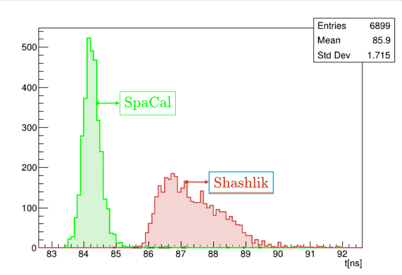
Measured timing of the photon cluster (\(t_{obs}\))
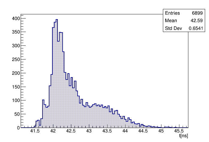
Calculated entry timing of the photons (\(t_{exp}\))
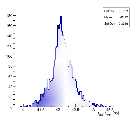
Resolution \(\text{SpaCal}\) \(t_{obs}-t_{exp}\)
\boxed{\text{SpaCal}}
\boxed{\text{Shashlik}}
Summary
Thank you!
- It was carried out a review of the most important aspects of the U1b and U2 LHCb calorimeters with a focus on the timing of the tracks.
- There were performed full ECAL simulations using the Hybrid-MC toolkit. The VELO reconstruction and both U1b and U2 configurations were considered in this study.
- Preliminary results include obtaining the entry time of the photons in the calorimeter using VELO and CALO information as well as the reconstructed time after full ECAL simulation.
-
Next steps:
- Examine PV positions after full simulation and analyze how to estimate their time using only ECAL timing
IJCLab internship report: U2 ECAL study
By Sebastian Ordoñez


