Visualizing the loss landscape of neural nets

Hao Li, Zheng Xu, Gavin Taylor, Christoph Studer, Tom Goldstein

(NIPS 2018)

What is the relationship between trainability, generalisation, and architecture choices?

• architecture choices \(\rightarrow\) loss landscape
• global loss landscape (convex or not) \(\leftrightarrow\) trainability
• landscape surrounding minima \(\rightarrow\) generalisation

Questions

Tricks of the trade

• Mini-batching
• Batch normalisation
• Self-normalisation
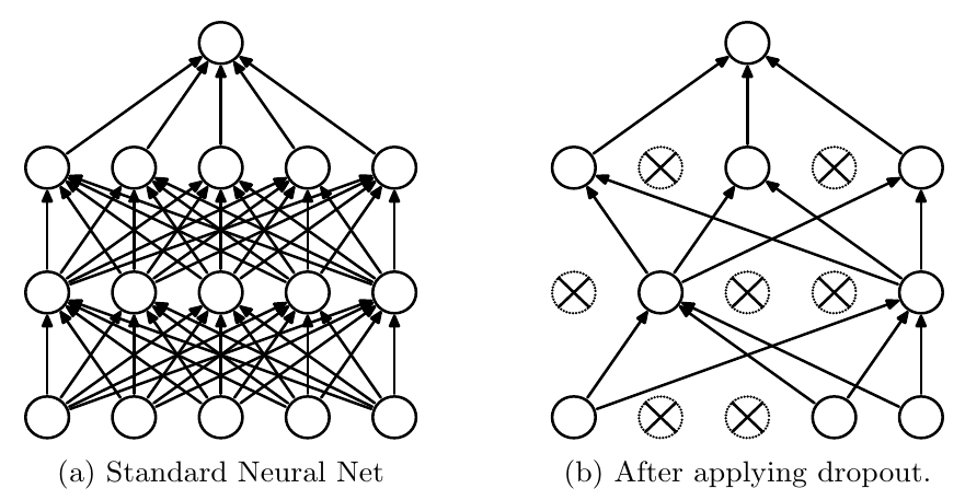
• Dropout
• Residual connections

Techniques for visualising

between two minima

Minimise \(L(\theta) = \frac{1}{m} \sum_{i=1}^m l(x_i, y_i; \theta)\)

\(x_i\) feature vectors

\(y_i\) labels

\(\theta\) model parameters

For two parameter sets \(\theta_1\) and \(\theta_2\),

plot \(f(\alpha) = L((1 - \alpha) \theta_1 + \alpha \theta_2)\)

Techniques for visualising

around one minimum

Around a parameter set \(\theta\):

• For 1D, choose a direction vector \(\delta\), and plot \( f(\alpha) = L(\theta + \alpha \delta) \)
• For 2D, choose two direction vectors \(\delta\) and \(\eta\), and plot \( f(\alpha, \beta) = L(\theta + \alpha \delta + \beta \eta) \)

Filter-wise normalisation

Direction vectors have same dimensionality as \(\theta\)

Normalise each direction vector filter-wise: \(d_{i,j} \leftarrow \frac{d_{i,j}}{||d_{i,j}||} ||\theta_{i,j}||\)

Test models

VGG (2014)

AlexNet (2012)

ResNet (2015)

Wide-ResNet (2016)

ResNet-noshort

DenseNet (2016)

Residual connections \(\leftrightarrow\) network depth

Residual connections \(\leftrightarrow\) network width

Does this capture convexity?

The principle curvatures of a randomly projected (Gaussian) surface are weighted averages of the principle curvatures of the original surface (with Chi-square coefficients)

So: non-convexity in the projected surface

\(\Longleftrightarrow\) non-positive projected Hessian eigenvalues

\(\Longrightarrow\) non-positive original Hessian eigenvalues

\(\Longleftrightarrow\) non-convexity in original surface

Visualising optimisation paths

In high dimension, random vectors are mostly orthogonal to anything independent (\(E[S_C(v_1, v_2)] \sim \sqrt{\frac{2}{\pi n}}\))

So random projections don't capture much

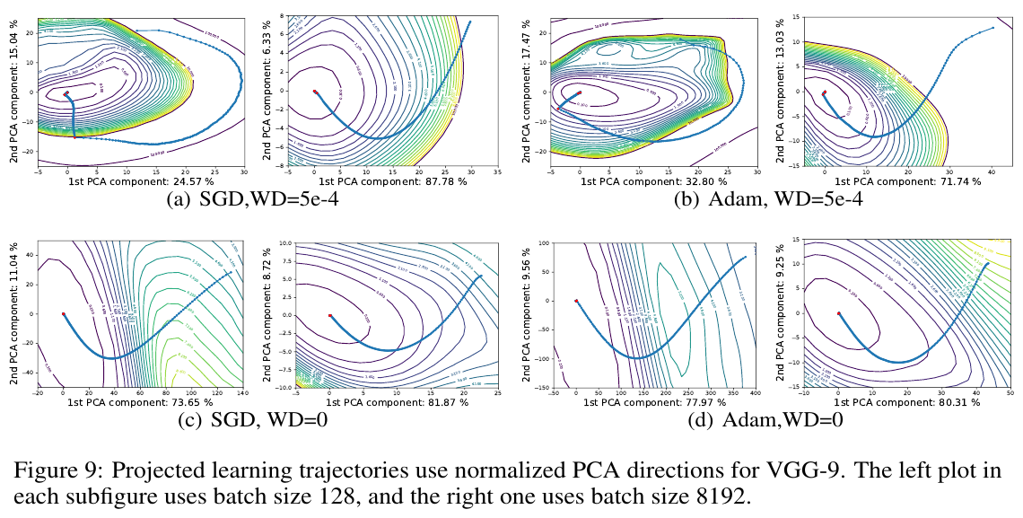
Visualising optimisation paths

use PCAs instead