1. Introduction to Causal Learning 

Background

• Machine learning and graphical causality were developed separately.

• Now, there are needs to integrate two methods and to find causal inference.

• A central problem for AI and causality is Causal Representation Learning — the discovery of high-level causal variables from low-level observations. 

Key research challenges with the Current ML Methods 

• Issue 1: Robustness 
• Issue 2: Learning Reusable mechanism 
• Issue 3: A Causality Perspective 

Key Research Challenges

• Issue 1: Robustness

  • In the real world, often little control over the distribution of observed data.

    • E.g., in computer vision, changes in variable distribution may come from aberrations like camera blur, noise, or compression quality.

  • There are several ways to test the generalization of classification, but no definitive consensus about the generalization

  • The causal model can be a way to handle these problems by using statistical dependences and distribution shifts, e.g., intervention. 

Key Research Challenges

• Issue 2: Learning reusable mechanism 

  • Repeating learning process every time whenever we learn new knowledge is waste of resources.

  • Need to re-use previous knowledge and skill in novel scenarios \(\to\) Modular representation

  • Modular representation behave similarly across different tasks and environments.

Key Research Challenges

Levels of causal modeling 

https://real-robot-challenge.com/

https://real-robot-challenge.com/

Physical modeling, differential equations:

\(F = ma\) 

\( a = \frac{d}{dt} v(t) \) 

\(v = \frac{d}{dt}s(t)\)

Levels of causal modeling 

https://real-robot-challenge.com/

statistical learning

Levels of causal modeling 

• Predicting in the i.i.d. setting

  • What is the probability that this particular image contains a dog?

  • What is the probability of heart failure given certain diagnostic measurements (e.g., blood pressure) carried out on a patient?

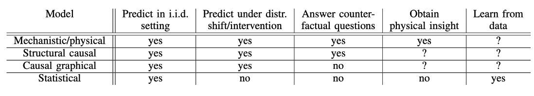
Levels of causal modeling 

• Predicting Under Distribution Shifts 

  • Is increasing the number of storks in a country going to boost its human birth rate?

  • Would fewer people smoke if cigarettes were more socially stigmatized?

Levels of causal modeling 

• Answering Counterfactual Questions 

  • Intervention: How does the probability of heart failure change if we convince a patient to exercise regularly?

  • Counterfactual: Would a given patient have suffered heart failure if they had started exercising a year earlier?

Levels of causal modeling 

• Learning from data 

  • Observational vs. Interventional data

    • E.g., images vs. experimental data (RCT)

  • Structured vs. Unstructured data

    • E.g., Principal Component Analysis (PCA) vs. raw data

Levels of causal modeling 

2. Causal representation learning 

Causal models and inference

1. Methods driven by i.i.d. data

2. The Reichenbach Principle: From Statistics to Causality

3. Structural Causal Models (SCMs)

4. Difference Between Statistical Models, Causal Graphical Models, and SCMs

Causal models and inference

• Methods driven by i.i.d. data

  • In many cases i.i.d. assumption can’t be guaranteed, e.g., selection bias \(\to\) Can't make  causal inferences

  • Mainly used for Statistical Inference Models

Causal models and inference

• The Reichenbach Principle (aka Common Cause Principle)

  • If two observables \(X\) and \(Y\) are statistically dependent, then there exists a variable \(Z\) that causally influences both and explains all the dependence in the sense of making them independent when conditioned on \(Z\).

• \(X \to Z \to Y\);     \(X \leftarrow Z \leftarrow Y\);     \(X \leftarrow Z \rightarrow Y\)

Causal models and inference

• The Reichenbach Principle (aka Common Cause Principle)

  • If two observables \(X\) and \(Y\) are statistically dependent, then there exists a variable \(Z\) that causally influences both and explains all the dependence in the sense of making them independent when conditioned on \(Z\).

• \(X \to Z \to Y\);     \(X \leftarrow Z \leftarrow Y\);     \(X \leftarrow Z \rightarrow Y\)

• Without additional assumptions, we can’t distinguish these three cases \(\to\) Observational distribution over \(X\) and \(Y\) is the same in all three cases

Causal models and inference

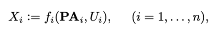
• Structural Causal Models (SCMs)

  • Consists of a set of random variable X with directed edges

    ●

  • The set of noises is assumed to be jointly independent.

  • The independence of noises allows causal factorization.

  • \(P(X_1, ..., X_n) = \prod_{i=1}^n P(X_i | \mathbf{PA}_i)\)

Causal models and inference

• Difference b/w Statistical Models, Causal Graphical Models, and SCMs

  • Statistical model:

    • Same conditional independence (Markov equivalence) \(\rightarrow \) insufficient for causal discovery

      • \(X \rightarrow Z \rightarrow Y\)

      • \(X \leftarrow Z \leftarrow Y\)

      • \(X \leftarrow Z \rightarrow Y\)

Causal models and inference

• Difference b/w Statistical Models, Causal Graphical Models, and SCMs

  • Causal Graphical Models

    • By using directed edges, can compute interventional distributions, e.g., disconnecting parents or fixing values

Causal models and inference

• Difference b/w Statistical Models, Causal Graphical Models, and SCMs

  • Structural Causal Models

    • Composed of a set of causal variables and a set of structural equations with noise variables \(U\).

    • Intervention and Counterfactuals

Causal models and inference

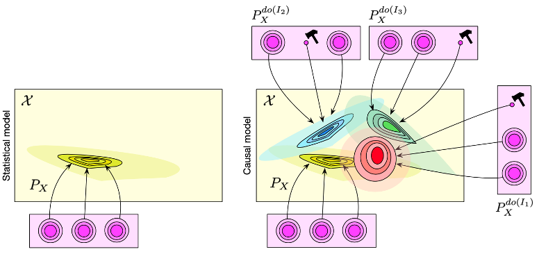
Difference b/w Statistical Models, Causal Graphical Models, and SCMs

3. Independent causal mechanisms 

Independent Causal Mechanisms (ICM)

The causal generative process of a system’s variables is composed of autonomous modules that do not inform or influence each other. In the probabilistic case, this means that the conditional distribution of each variable given its causes (i.e., its mechanism) does not inform or influence the other mechanisms.

 

• To correctly predict the effect of intervention, it needs to be robust during distribution shift, e.g., generalizing from an observational distribution to interventional distributions.

Independent Causal Mechanisms (ICM)

Applying ICM to causal factorization \(P(X_1, ..., X_n) = \prod_{i=1}^n P(X_i | \mathbf{PA}_i)\) implies that factors should be independent in the sense that 

1. intervening upon one mechanism \(P(X_i | \mathbf{PA}_i)\) does not change any of the other mechanisms \(P(X_j | \mathbf{PA}_j)\), \(j \neq i \)
    
2. knowing some other mechanisms \(P(X_i | \mathbf{PA}_i)\), \(i \neq j\), does not give us information about mechanism \(P(X_j | \mathbf{PA}_j)\) 

Sparse Mechanism Shift (SMS)

Small distribution changes tend to manifest themselves in a sparse or local way in the causal/disentangled factorization, i.e., they should usually not affect all factors simultaneously.

Recall: causal/disentangled factorization is
\(P(X_1, ..., X_n) = \prod_{i=1}^n P(X_i | \mathbf{PA}_i)\)

Sparse Mechanism Shift (SMS)

• Intellectual descendant of Simon's invariance criterion, i.e., that the causal structure remains invariant across changing background conditions 

• SMS has been recently used to learn causal models, modular architectures, and disentangled representations 

4. Causal discovery and machine learning 

Review: two assumptions 

1. Causal Markov assumption: Upon accurately specifying a causal graph \(\mathcal{G}\) among some set of variables \(V\) (in which \(V\) includes all the common causes of pairs in \(V\)), at least the independence relations obtained by applying \(d\)-separation to \(\mathcal{G}\) hold in the population probability distribution over \(V\).
2. Causal Faithfulness assumption: exactly the independence relations obtained by applying \(d\)-separation to \(\mathcal{G}\) hold in the probability distribution over \(V\).

Challenges of causal discovery

1. Given finite data sets, conditional independence testing is hard without additional assumptions 
2. With only two variables, there is no conditional independence → we don't know the direction of causation 

If we make assumptions about the function class \(f\), we can solve the above two challenges. 

Nevertheless, more often than not, causal variables are not given and need to be learned. 

5. Learning causal variables 

But first,
what is representation learning? 

• In ML, in order to train a model, we must choose the set of features that best represent the data. 

representation

• Representation learning is a class of machine learning approaches that allow a system to discover the representations required for feature detection of classification from raw data 
• Representation learning works by reducing high-dimensional data to low-dimensional data

Example: causal representation learning problem setting 

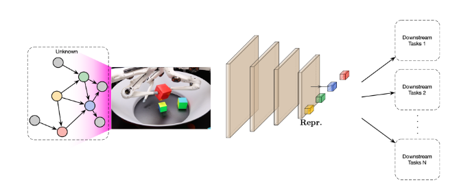
unknown causal structure

observed data \(X\) 

Identifiability guarantees for causal disentanglement from soft interventions

• What is causal disentanglement? 
  • ... seeks to recover a causal representation in latent space, i.e., a small number of variables \(U\) that are mapped to the observed samples in the ambient space via some mixing map \(f\) 
• What is a soft intervention? 
• What can be identified? 

Identifiability guarantees for causal disentanglement from soft interventions

Formally: 

• observed variables \(X = (X_1, ..., X_n)\) are generated from latent variables \(U = (U_1, ..., U_p)\) through an unknown deterministic mixing function \(f\) 

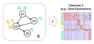
\(U\) factorizes according to unknown DAG \(\mathcal{G}\). 

Q: How many nodes does \(\mathcal{G}\) have? 

Identifiability guarantees for causal disentanglement from soft interventions

• Consider atomic (i.e., single-node) interventions on the latent variables \(U\) 
• An intervention \(I\) modifies the joint distribution of latent variables \(\mathbb{P}_U\) by changing the conditional distribution of \(\mathbb{P}(U_i|U_{PA(i)})\)
  • A hard intervention removes the dependency of \(U_i\) on its parents 
  • A soft intervention preserves dependency but changes the conditional distribution \(\mathbb{P}(U_i|U_{PA(i)})\) to  \(\mathbb{P}^I(U_i|U_{PA(i)})\)

Identifiability guarantees for causal disentanglement from soft interventions

• Given unpaired data from observational and interventional distributions \(\mathcal{D}, \mathcal{D}^{I_1}, ..., \mathcal{D}^{I_K}\) where \(\mathcal{D}\) denotes samples of \(X = f(U)\) and the rest are interventional distributions 
• focus on scenario where we have at least one intervention per latent node 
• latent variables \(U\), dimension \(p\), the DAG \(\mathcal{G}\) and interventional targets \(I_1, ... =, I_K\) are all unknown.
• Goal: identify \(U, \mathcal{G}, I_1, ..., I_K\) given \(X\) in  \(\mathcal{D}, \mathcal{D}^{I_1}, ..., \mathcal{D}^{I_K}\)

Identifiability guarantees for causal disentanglement from soft interventions

• Without making further assumptions on the form of \(f\), the latent model can be identified up to the equivalence class of latent models that can generate the same observed samples of \(X\) in \(\mathcal{D}, \mathcal{D}^{I_1}, ..., \mathcal{D}^{I_K}\)
• The main result of this paper is the identifiability guarantee for causal disentanglement from soft interventions 
  • i.e., sets of \(U, \mathcal{G}, I_1, ..., I_K\) for the same \(X\) 
• They also developed an autoencoding variational Bayes algorithm 

Three problems of modern ML 

... in light of causal representation learning 

1. Learning disentangled representation 
2. Learning transferable mechanisms 
3. Learning interventional world models and reasoning 

1. Learning disentangled representation 

ICM Principle implies

• independence of the SCM noise terms in \(X_i := f_i(\mathbf{PA}_i, U_i)\) and
• feasibility of the disentangled representation \(P(S_1, ..., S_n) = \prod_{i=1}^n P(S_i | \mathbf{PA}_i)\) and
• the property that the conditionals \(P(S_i | \mathbf{PA}_i)\) are independently manipulable and largely invariant across related problems. 

1. Learning disentangled representation 

Problem: Given data \(X = (X_1, \ldots, X_d)\), construct causal variables \(S_1, ..., S_n (n \ll d)\) and mechanisms \(S_i := f_i(\mathbf{PA}_i, U_i)\) 

Step 1: Use an encoder \(q: \mathbb{R}^d \to \mathbb{R}^n\) to take \(X\) into a latent representation 

Step 2: mapping \(f(U)\) determined by structural assignments \(f_1, ..., f_n\) 

Step 3: Apply a decoder \(p: \mathbb{R}^n \to \mathbb{R}^d\)

1. Learning disentangled representation 

• Much existing work in disentanglement focus on a special case, independent factors of variation.
  • i.e., \(\forall i, S_i := f_i(U_i)\) where \(U_i\) are independent exogenous noise variables
• Which factors of variation can be disentangled depend on which interventions can be observed  
• When learning causal variables from data, which variables can be extracted and their granularity depends on which distribution shifts, explicit interventions, and other supervision signals available 

2. Learning transferable mechanism 

• The world is modular, in the sense that mechanisms of the world play roles across a range of environments, tasks, and settings
• For pattern recognition tasks, existing works suggest the learning causal models that contain independent mechanisms may help in transferring modules across substantially different domains 

3. Learning interventional world models 

• We need to go beyond deep learning which learns representations of data that preserve relevant statistical properties
• Instead, we should be learning interventional world models, models that support interventions, planning, and reasoning.
• Konrad Lorenz's Die Rückseite des Spiegels (i.e., Behind the Mirror: A search for natural history of human knowledge).
  • thinking as acting in an imagined space 
  • the need for representing oneself in this imagined space 
  • free will as a means to communicate about actions take by the "self" variable \(\to\) social and cultural learning 

Semi-supervised learning (SSL)

• In supervised learning, we receive \(n\) i.i.d. data points from the joint distribution: \((\mathbf{X}_1, Y_1), \ldots, (\mathbf{X}_n, Y_n) \sim P(\mathbf{X}, Y)\) 
• In semi-supervised learning, we receive \(m\) additional unlabeled data points: \(\mathbf{X}_{n+1}, \ldots, \mathbf{X}_{n+m} \sim P(\mathbf{X})\) 
• ML model is causal if we predict effect from cause 
• ML model is anti-causal if we predict cause from effect
• For a causal learning problem (i.e., predicting effect \(Y\) from cause \(\bf X\)), SSL would not work  
  • In other words, SSL only works in the anti-causal direction 
• Why will SSL not work? 

Semi-supervised learning (SSL)

• Task: predict label \(y\) for some specific feature vector \(x\) 
• Knowledge of \(P(X)\) (obtained through additional unlabelled data) does not help if the causal direction is \(X \to Y\). Why?  
  • ICM principle. 
• Not all hope is lost though - knowing \(P(X)\) is still helpful, as it can help us select a predictor with a lower risk 
  • ... by helping us identify the least common \((x, y)\) pairs and appearing in the weighting function 

Semi-supervised learning (SSL)

• \(P(\text{cause, effect}) = P(\text{cause}) P(\text{effect} | \text{cause}) \)
• We've already seen that \(P(\text{cause})\) gives us no information about \(P(\text{effect}|\text{cause})\) 
• ICM principle also tells us that when the joint distribution \(P(\text{cause, effect})\) changes across different sets, the change of \(P(\text{cause})\) doesn't tell us anything about the change of \(P(\text{effect}|\text{cause})\) 
  • i.e., \(P(\text{effect}|\text{cause})\) might as well remain unchanged 
  • using this assumption in ML is known as covariate shift

Semi-supervised learning (SSL)

• If features \(X\) correspond to cause and labels \(Y\) correspond to effect: 
  • Having more unlabelled data only gives us information on \(P(\bf X)\) but doesn't tell us anything about \(P(Y|\bf{X})\)
• If features \(X\) correspond to effect and labels \(Y\) correspond to cause: 
  • information on \(P(X)\) may tell us more about \(P(Y|X)\)

Semi-supervised learning (SSL)

• If \(\mathbf{X} \to Y\): 
  • causal factorization: \[P(\mathbf{X}, Y) = P(\mathbf{X}) \times P(Y | \mathbf{X}) \]
  • ICM principle tells us that \(P(\mathbf{X})\) gives no information about \(P(Y | \mathbf{X})\) \(\implies\) Having an additional \(m\) points only gives me information about \(P(\mathbf{X})\) and not about \(P(Y|\mathbf{X})\) 
• If \(\mathbf{X} \leftarrow Y\):  
  • causal factorization: \[P(\mathbf{X}, Y) = P(Y) \times P(\mathbf{X} |Y) \]

Adversarial vulnerability 

Neural networks are "brittle" against adversarial attacks. 

https://arxiv.org/pdf/1312.6199.pdf

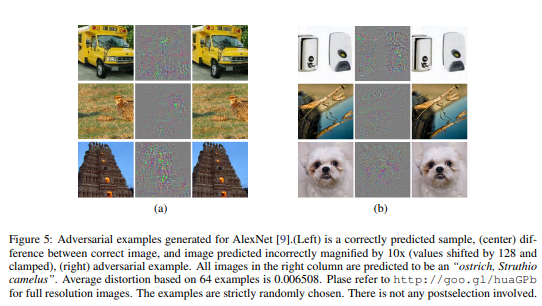
Adversarial vulnerability 

• How are these adversarial attacks found? 
  • By exploiting the fact that human visual robustness \(\neq\) robustness of classifiers obtained through statistical machine learning 
  • find an example which leads to maximal changes in the classifier's output, subject to the constraint that they lie in an \(l_p\) ball in the pixel space 
• How can we guard against such adversarial attacks? 

Adversarial vulnerability 

• How can we guard against such adversarial attacks? 
  • Method 1: Reconstruct the input by an auto-encoder before feeding it to a classifier 
  • Method 2: Solve the anti-causal classification problem by modeling the causal generative direction 
• If the predictor approximates the causal mechanism (that is inherently transferable and robust), adversarial examples should be harder to find 

Robustness and strong generalization 

• Example: credit scoring
  • Classification with strategic agents 
  • strategic action 1: change their current debt by paying it off \(\implies\) more likely to influence the prob of paying back 
  • strategic action 2: move to a more affluent neighborhood \(\implies\) less likely to influence prob of paying back 
• We could build a scoring system that is more robust to strategic behavior by only using causal features as inputs

Out-of-distribution (OOD) generalization 

• Empirical risk minimization set-up: 
  • data from a joint distribution \(\mathcal{D} = P(\mathbf{X}, Y)\) 
  • Goal: find predictor \(g \in \mathcal{H}\) to minimize empirical risk \(\hat{R}_\mathcal{D} (g) = \mathbb{E}_\mathcal{D}[\text{loss}(Y, g(Y)]\)  
• OOD generalization: small expected loss with different distribution \( \mathcal{D}^{'}\)  
  • \(R^{OOD}(g) = \mathbb{E}_{\mathcal{D}^{'}}[\text{loss}(Y, g(Y)]\)
• Ideally, we want \(R^{OOD}(g)\) to track the performance of \(\hat{R}_{\mathcal{D}}(g)\) 

Out-of-distribution (OOD) generalization 

• We could restrict  \( \mathcal{D}^{'}\) to be the result of a certain set of interventions 
• The worst case OOD risk then becomes \[ R^{OOD}_{\mathbb{P}_\mathcal{G}} = \max_{\mathcal{D}^{'} \in\mathbb{P}_\mathcal{G} } \mathbb{E}_{\mathcal{D}^{'}} [\text{loss}(Y, g(X)] \]
• To learn a robust predictor (for different environments that could give rise to distribution shifts), we solve \[g^* = \arg\min_{g \in \mathcal{H}} \max_{\mathcal{D}^{'} \in \mathcal{E} } \mathbb{E}_{\mathcal{D}^{'}} [\text{loss}(Y, g(X)]  \] where \(\mathcal{E} \subset \mathbb{P}_\mathcal{G}\). 
  • If \(\mathcal{E}\) does not coincide with \(\mathbb{P}_\mathcal{G}\) then we might still get arbitrarily large estimation error in the worst case 

Other implications for machine learning 

Scientific applications

• Causal inference could be helpful in scenarios that lack systematical experimental condition, such as health care 

Multi-task learning and continual learning 

• Multi-task learning: building a system that can solve multiple tasks across different environments 

Summary 

• Main point: machine learning can benefit from integrating causal concepts 
• Make a weaker assumption that the iid assumption: the data on which the model will be applied comes from a possibly different distribution but involving (mostly) the same causal mechanisms 

Questions / Comments?

Thank you for listening!