

Lecture 1: Intro and Linear Regression
Intro to Machine Learning

Welcome to 6.390!
Outline
- Course Overview
- Team, logistics, and topics overview
- Supervised learning, terminologies
- Ordinary least square regression
- Formulation
- Closed-form solutions
Team


~50 awesome LAs
Class meetings
assignments
Hours:
Lec: 1.5 hr
Rec + Lab: 3 hr
Notes + exercise: 2 hr
Homework: 6-7 hr

A nominal content week:
mix of theory, concepts, and application to problems!
-
Exercises: Releases on Thursday 9am, due the following Tuesday 9am.
Relatively easy questions based on that week’s lecture and notes reading. -
Lecture: Thursday, 11am–12:30pm, 10-250. Recorded.
Overview the technical contents, and tie together the high-level motivations, concepts, and stories. -
Recitation: Friday, various sections. See introml for exact time.
Assumes you have read and done exercises; start on homework. -
Homework: Releases Friday 9am; due Wed. (12 days later) at 11:59pm
Harder questions: concepts, mechanics, implementations. -
Lab: Tuesdays, various sections. Synchronous. See website for exact time and room. In-class empirical exploration of concepts, work with partner(s) on questions, Check-off conversation with staff member.
Grading and collaboration
- Our objective (and we hope yours) is for you to learn about machine learning
- take responsibility for your understanding
- we are here to help!
- Grades formula: exercises 5% + homework 20% + labs 15% + midterm 30% + final 30%
- Lateness: 20% penalty per day, applied linearly (so 1 hour late is -0.83%)
- Extensions:
- 20 one-day extensions (extend one assignment's deadline by one full day), will be applied automatically at the end of the term in a way that is maximally helpful
Grading and collaboration
- Midterm 1: Wednesday, October 8, 730pm-9pm
- Midterm 2: Wednesday, Nov 12, 730pm-9pm
- Final: scheduled by Registrar (posted in 3rd week). ⚠️ – might be as late as Dec 19!
Detailed exam logistics will be posted 3 weeks before the exam date.
- Collaboration:
- Understand everything you turn in
- Coding and detailed derivations must be done by you
- See collaboration policy/examples on course web site
How to get help
- Office hours: lots! (Starting Wed Sept 10)
- Schedule details on OHs page (includes instructors' OHs)
- See Calendar page for holiday/schedule shift
- Make use of Piazza and Pset-partners!
- Logistic, personal issues, reach out to 6.390-personal@mit.edu (looping in S^3 and/or DAS)
Expected prerequisite background
Things we expect you to know (we use these constantly, but don’t teach them explicitly):
- Programming (e.g. as in 6.101[009] or 6.121[006])
- Intermediate Python, including classes
- Exposure to algorithms – ability to understand & discuss pseudo-code, and implement in Python
- Linear Algebra (e.g. as in 18.06, 18.C06, 18.03, or 18.700)
- Matrix manipulations: transpose, multiplication, inverse etc.
- Points and planes in high-dimensional space
- (Together with calculus): taking gradients, matrix calculus
What we're teaching: Machine Learning
Given:
- a collection of examples (gene sequences, documents, …)
- an encoding of those examples in a computer (as vectors)
Derive:
- a computational model that describes relationships within and among the examples that is expected to characterize well new examples from that same population, to make good predictions or decisions
A model might:
- classify images of cells as to whether they're cancerous
- specify groupings (clusters) of documents that address similar topics
- steer a car appropriately given lidar images of the surroundings
traditionally
supervised learning
unsupervised learning
reinforcement learning
nowadays
reinforcement learning
supervised learning
unsupervised learning
- self-supervised
- contrastive learning (DALLE)
- behavior cloning
RLHF (ChatGPT etc.)
- inverse reinforcement learning
Toddler demo, Russ Tedrake thesis, 2004
(Uses vanilla policy gradient (actor-critic))
Optimization + first-principle physics
DARPA Robotics Competition
2015
In 6.390:
supervised learning
unsupervised learning
reinforcement learning
- Intro to ML
- Regularization
- Gradient Descent
- Linear Classification
- Features, Neural Networks I
- Neural Networks II (Backprop)
- Convolutional Neural Networks
- Representation Learning
- Transformers
- Non-parametric Models
- Markov Decision Processes
- Reinforcement Learning
Topics in order:
supervised
unsupervised
reinforcement
Model class:
- linear models
- linear model on non-linear features
- fully connected feed-forward nets
- convolutional nets
- transformers
- Q-table
- tree, k-nearest neighbor, k-means
Optimization:
- analytical solutions
- gradient descent
- back propagation
- value iteration, Q-learning
- non-parametric methods
Learning process:
- training/validation/testing
- overfitting/underfitting
- regularization
- hyper parameters
Modeling choices:
- Supervised:
- regression
- classification
- Unsupervised/self-supervised
- Reinforcement/sequential
Many other ways to dissect
[These lists are neither exhaustive nor exclusive.]
Outline
- Course Overview
- Supervised learning, terminologies
- Ordinary least square regression
- Formulation
- Closed-form solutions
We first focus on an instance of supervised learning known as regression.
example: city daily energy consumption prediction
| Features | Label | |
|---|---|---|
| City | Temperature (°C) |
Energy used (GWh) |
| Chicago | 25 | 51 |
| New York | 28 | 57 |
| Boston | 31 | 63 |
| San Diego | 35 | 71 |
temperature \(x_1\)
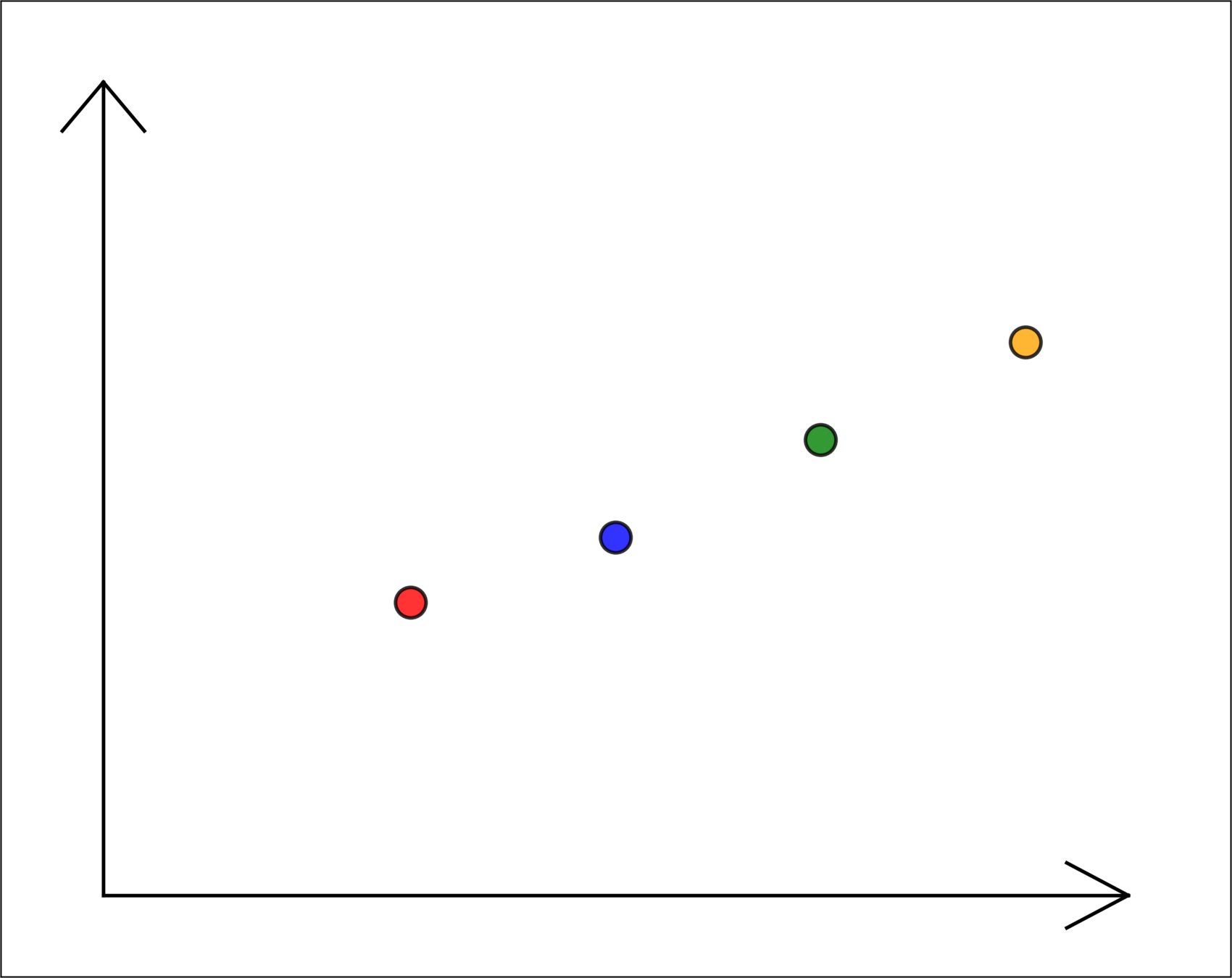
energy used \(y\)
toy data, for illustration only
Training data:
\(x^{(1)} =\begin{bmatrix} x_1^{(1)} \\[4pt] x_2^{(1)} \\[4pt] \vdots \\[4pt] x_d^{(1)} \end{bmatrix} \in \mathbb{R}^d\)
label
feature vector
\(y^{(1)} \in \mathbb{R}\)
\(\mathcal{D}_\text{train}:=\)
\(\left\{\left(x^{(1)}, y^{(1)}\right), \dots, \left(x^{(n)}, y^{(n)}\right)\right\}\)
\(n = 4, d = 1\)
\(n = 4 ,d = 2\)
temperature \(x_1\)
energy used \(y\)
temperature \(x_1\)
population \(x_2\)
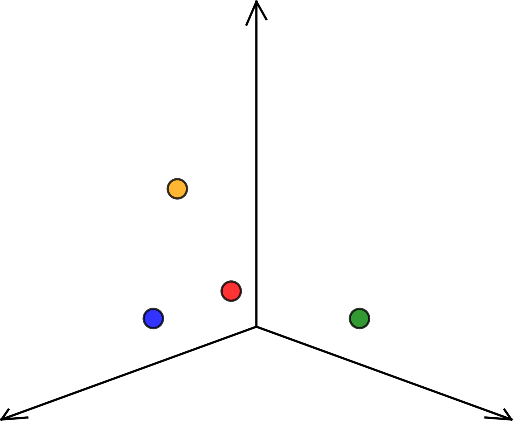
energy used \(y\)
Training data:
\(x^{(1)} =\begin{bmatrix} x_1^{(1)} \\[4pt] x_2^{(1)} \\[4pt] \vdots \\[4pt] x_d^{(1)} \end{bmatrix} \in \mathbb{R}^d\)
label
feature vector
\(y^{(1)} \in \mathbb{R}\)
\(\mathcal{D}_\text{train}:=\)
\(\left\{\left(x^{(1)}, y^{(1)}\right), \dots, \left(x^{(n)}, y^{(n)}\right)\right\}\)
\(n = 4 ,d = 2\)
temperature \(x_1\)
population \(x_2\)
energy used \(y\)
\((x^{(1)}, y^{(1)})\)
\(=\left(\begin{bmatrix} x_1^{(1)} \\[4pt] x_2^{(1)} \\[4pt] \end{bmatrix}, y^{(1)}\right)\)
\boxed{h}
Regression
Algorithm
💻
\rightarrow
\downarrow
y
x
\downarrow
\(\in \mathbb{R}^d \)
\(\in \mathbb{R}\)
\(\mathcal{D}_\text{train}\)
\rightarrow
\(\left\{\left(x^{(1)}, y^{(1)}\right), \dots, \left(x^{(n)}, y^{(n)}\right)\right\}\)
What do we want from the regression algortim?
A good way to label new features, i.e. a good hypothesis.
Suppose our friend's algorithm proposes \(h(x)=10\)
hypothesis
- Is this a hypothesis?
- Is this a "good" hypothesis? Or, what would be a "good" hypothesis?
- What can affect if and how we can find a "good" hypothesis?
- Loss
\(\mathcal{L}\left(h\left(x^{(i)}\right), y^{(i)}\right) \)
temperature \(x\)
\(h(x)=10\)
e.g. \(h\left(x^{(4)}\right) - y^{(4)} \)
energy used \(y\)
\(\mathcal{E}_{\text {train }}(h)=\frac{1}{n} \sum_{i=1}^n \mathcal{L}\left(h\left(x^{(i)} \right), y^{(i)}\right)\)
- Training error
e.g. with squared loss, the training error is the mean-squared-error (MSE)
e.g. squared loss \(\mathcal{L}\left(h\left(x^{(i)}\right), y^{(i)}\right) = (h\left(x^{(i)}\right) - y^{(i)} )^2\)
\(\mathcal{E}_{\text {test }}(h)=\frac{1}{n^{\prime}} \sum_{i=n+1}^{n+n^{\prime}} \mathcal{L}\left(h\left(x^{(i)}\right), y^{(i)}\right)\)
- Test error
\(n'\) unseen data points, i.e.
test data
set of \(h\) we ask the algorithm to search over
Hypothesis class \(\mathcal{H}:\)
\(\{\)constant functions\(\}\)
temperature \(x\)
energy used \(y\)
\(\subset\)
less expressive
more expressive
\(\{\)linear functions\(\}_1\)
1. technically, affine functions. ppl tend to be flexible about this terminology in ML.
\(h_1(x)=10\)
\(h_2(x)=20\)
\(h_3(x)=30\)
temperature \(x\)
energy used \(y\)
\(h(x)=\theta x + \theta_0\)
\boxed{h}
Regression
Algorithm
💻
\rightarrow
\downarrow
y
x
\downarrow
\(\in \mathbb{R}^d \)
\(\in \mathbb{R}\)
\(\mathcal{D}_\text{train}\)
\rightarrow
\(\left\{\left(x^{(1)}, y^{(1)}\right), \dots, \left(x^{(n)}, y^{(n)}\right)\right\}\)
hypothesis
🧠
- hypothesis class
- loss function
- ...
- Supervised learning
- Regression
- Training data, test data
- Features, label
- Loss function, training error, test error
- Hypothesis, hypothesis class
Quick summary
Outline
- Course Overview
- Supervised learning, terminologies
-
Ordinary least square regression
- Formulation
- Closed-form solutions
- Linear hypothesis class:
\(h\left(x ; \theta\right)\)
\( = \left[\begin{array}{lllll} \theta_1 & \theta_2 & \cdots & \theta_d\end{array}\right]\) \(\left[\begin{array}{c} x_1 \\ x_2 \\ \vdots \\ x_d\end{array}\right]\)
parameters
Linear least square regression
- Squared loss function:
\(\mathcal{L}\left(h\left(x^{(i)}\right), y^{(i)}\right) =(\theta^T x^{(i)}- y^{(i)} )^2\)
temperature \(x_1\)
population \(x_2\)
energy used \(y\)
for now, ignoring the offset
\(=\)
\(x\)
\(\theta^T\)
features
- MSE training error:
| Features | Label | ||
|---|---|---|---|
| City | Temperature | Population | Energy Used |
| Chicago | 90 | 7.2 | 45 |
| New York | 20 | 9.5 | 32 |
| Boston | 35 | 8.4 | 99 |
| San Diego | 18 | 4.3 | 39 |
\quad J(\theta_1, \theta_2) = \frac{1}{4}[
(\theta_1 \cdot 90 + \theta_2 \cdot 7.2 - 45)^2 \\
+ (\theta_1 \cdot 18 + \theta_2 \cdot 4.3 - 39)^2]
+ (\theta_1 \cdot 20 + \theta_2 \cdot 9.5 - 32)^2 \\
+ (\theta_1 \cdot 35 + \theta_2 \cdot 8.4 - 99)^2 \\
- \(J\) denotes training error, sometimes the more explicitly \(J(\theta; \text{data})\)
- want a more compact way to write this out
\quad J(\theta_1, \theta_2) = \frac{1}{4}[
(e_1^2+e_2^2+e_3^2+e_4^2) ]\\
| Features | Label | ||
|---|---|---|---|
| City | Temperature | Population | Energy Used |
| Chicago | 90 | 7.2 | 45 |
| New York | 20 | 9.5 | 32 |
| Boston | 35 | 8.4 | 99 |
| San Diego | 18 | 4.3 | 39 |
\(X =\begin{bmatrix}90 & 7.2 \\20 & 9.5\\35 & 8.4 \\18 & 4.3\end{bmatrix}\)
\(Y =\begin{bmatrix}45 \\32 \\99 \\39\end{bmatrix}\)
\(\theta =\begin{bmatrix}\theta_1 \\\theta_2\end{bmatrix}\)
\(X = \begin{bmatrix}x_1^{(1)} & \dots & x_d^{(1)}\\\vdots & \ddots & \vdots\\x_1^{(n)} & \dots & x_d^{(n)}\end{bmatrix}\)
\(Y = \begin{bmatrix}y^{(1)}\\\vdots\\y^{(n)}\end{bmatrix}\)
\(\theta = \begin{bmatrix}\theta_{1}\\\vdots\\\theta_{d}\end{bmatrix}\)
\( J(\theta) =\frac{1}{n}({X} \theta-{Y})^{\top}({X} \theta-{Y})\)
Let
Then
\(\in \mathbb{R}^{n\times d}\)
\(\in \mathbb{R}^{n\times 1}\)
\(\in \mathbb{R}^{d\times 1}\)
\(\in \mathbb{R}^{1\times 1}\)
e.g.
| Features | Label | ||
|---|---|---|---|
| City | Temperature | Population | Energy Used |
| Chicago | 90 | 7.2 | 45 |
| New York | 20 | 9.5 | 32 |
| Boston | 35 | 8.4 | 99 |
| San Diego | 18 | 4.3 | 39 |
\( J(\theta) =\frac{1}{n}({X} \theta-{Y})^{\top}({X} \theta-{Y})\)
\(X =\begin{bmatrix}90 & 7.2 \\20 & 9.5\\35 & 8.4 \\18 & 4.3\end{bmatrix}\)
\(Y =\begin{bmatrix}45 \\32 \\99 \\39\end{bmatrix}\)
deviation
\(\theta =\begin{bmatrix}\theta_1 \\\theta_2\end{bmatrix}\)
training error (MSE):
\( {X} \theta - Y\)
summing deviation squared
\(= \begin{bmatrix}90\theta_1 + 7.2\theta_2 - 45 \\20\theta_1 + 9.5\theta_2 - 32 \\35\theta_1 + 8.4\theta_2 - 99 \\18\theta_1 + 4.3\theta_2 - 39\end{bmatrix}\)
= \(({X} \theta-{Y})^{\top}({X} \theta-{Y})\)
\(= \begin{bmatrix}e_1 \\e_2\\e_3\\e_4\end{bmatrix}\)
e_1^2+e_2^2+e_3^2+e_4^2
\(=\begin{bmatrix}e_1, e_2, e_3, e_4\end{bmatrix}\begin{bmatrix}e_1 \\e_2\\e_3\\e_4\end{bmatrix}\)
want to show:
Outline
- Course Overview
- Supervised learning, terminologies
-
Ordinary least square regression
- Formulation
- Closed-form solutions
- Q: What kind of function is \(J(\theta)\)?
- A: Quadratic function
- Q: What does \(J(\theta)\) look like?
- A: Typically, looks like a "bowl"
- Q: How to find the minimizer?
Objective function (training error)
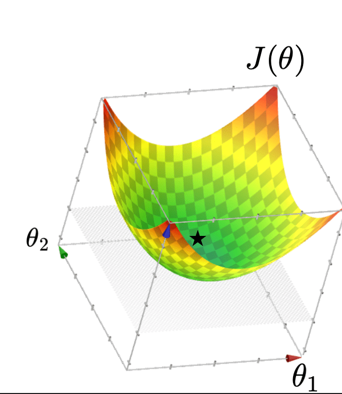
\( J(\theta) =\frac{1}{n}({X} \theta-{Y})^{\top}({X} \theta-{Y})\)
[1d case walk-through on board]
goal: find \(\theta\) to minimize \(J(\theta)\)
For \(f: \mathbb{R}^m \rightarrow \mathbb{R}\), its gradient \(\nabla f: \mathbb{R}^m \rightarrow \mathbb{R}^m\) is defined at the point \(p=\left(x_1, \ldots, x_m\right)\) as:
\nabla f(p)=\left[\begin{array}{c}
\frac{\partial f}{\partial x_1}(p) \\
\vdots \\
\frac{\partial f}{\partial x_m}(p)
\end{array}\right]
Sometimes the gradient is undefined or ill-behaved, but today it is well-behaved.
- The gradient generalizes the concept of a derivative to multiple dimensions.
- By construction, the gradient's dimensionality always matches the function input.
\nabla f(p)=\left[\begin{array}{c}
\frac{\partial f}{\partial x_1}(p) \\
\vdots \\
\frac{\partial f}{\partial x_m}(p)
\end{array}\right]
3. The gradient can be symbolic or numerical.
f(x, y, z) = x^2 + y^3 + z
example:
its symbolic gradient:
just like a derivative can be a function or a number.
evaluating the symbolic gradient at a point gives a numerical gradient:
\nabla f(x, y, z) = \begin{bmatrix}
2x \\
3y^2 \\
1
\end{bmatrix}
\nabla f(3, 2, 1) = \nabla f(x,y,z)\Big|_{(x,y,z)=(3,2,1)} = \begin{bmatrix}6\\12\\1\end{bmatrix}
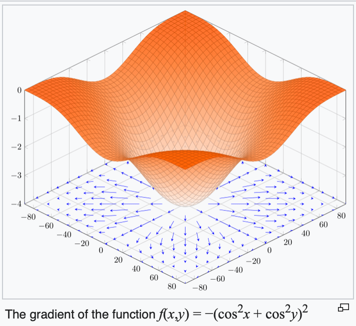
4. The gradient points in the direction of the (steepest) increase in the function value.
\(\frac{d}{dx} \cos(x) \bigg|_{x = -4} = -\sin(-4) \approx -0.7568\)
\(\frac{d}{dx} \cos(x) \bigg|_{x = 5} = -\sin(5) \approx 0.9589\)
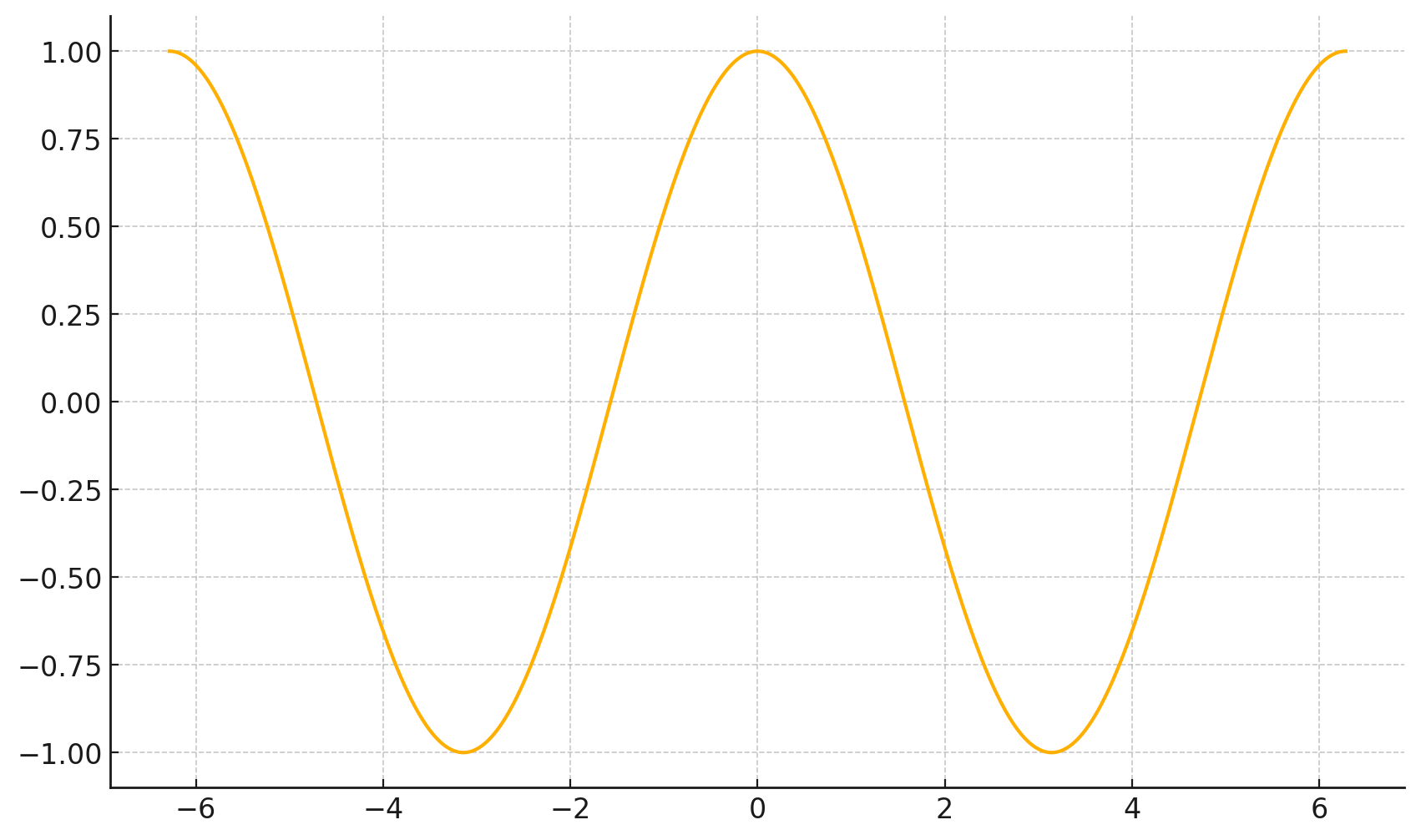
f(x)=\cos(x)
x
5. The gradient at the function minimizer is necessarily zero
f(x)=\cos(x)
x
- Typically, \(J(\theta)=\frac{1}{n}({X} \theta-{Y})^{\top}({X} \theta-{Y})\) "curves up"
- The minimizer of \(J(\theta)\) necessarily has a gradient zero
- Set the gradient \(\nabla_\theta J\stackrel{\text { set }}{=} 0\)
\(\nabla_\theta J=\left[\begin{array}{c}\partial J / \partial \theta_1 \\ \vdots \\ \partial J / \partial \theta_d\end{array}\right]\)
= \(\frac{2}{n}\left(X^T X \theta-X^T Y\right)\)
\Rightarrow
\(\theta^*=\left({X}^{\top} {X}\right)^{-1} {X}^{\top} {Y}\)
- When \(\theta^*\) is well defined, it's indeed guaranteed to be the unique minimizer of \(J(\theta\))
- Closed-form solution, does not feel like "training"
- The very rare case where we get such a general and clean solution with nice theoretical guarantee.
\(\theta^*=\left({X}^{\top} {X}\right)^{-1} {X}^{\top} {Y}\)
Beauty of
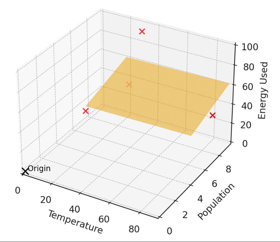
1. "center" the data
How to deal with \(\theta_0\)?
when data is centered, the optimal offset is guaranteed to be 0
centering
| Features | Label | ||
|---|---|---|---|
| City | Temperature | Population | Energy Used |
| Chicago | 90 | 7.2 | 45 |
| New York | 20 | 9.5 | 32 |
| Boston | 35 | 8.4 | 100 |
| San Diego | 18 | 4.3 | 39 |
\Downarrow
| Features | Label | ||
|---|---|---|---|
| City | Temperature | Population | Energy Used |
| Chicago | 49.25 | -0.15 | -9.00 |
| New York | -20.75 | 2.15 | -22.00 |
| Boston | -5.75 | 1.05 | 46.00 |
| San Diego | -22.75 | -3.05 | -15.00 |
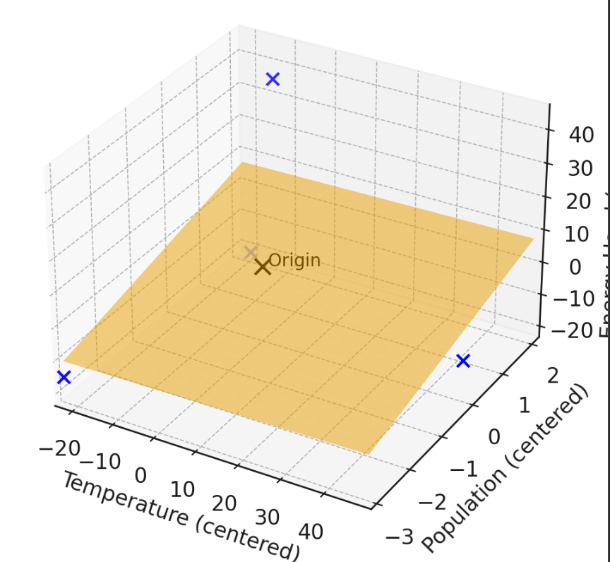
all column-wise \(\Sigma =0\)

2. Append a "fake" feature of \(1\)
\(h\left(x ; \theta, \theta_0\right)=\theta^T x+\theta_0\)
\( = \left[\begin{array}{lllll} \theta_1 & \theta_2 & \cdots & \theta_d\end{array}\right]\) \(\left[\begin{array}{l}x_1 \\ x_2 \\ \vdots \\ x_d\end{array}\right] + \theta_0\)
\( = \left[\begin{array}{lllll} \theta_1 & \theta_2 & \cdots & \theta_d & \theta_0\end{array}\right]\) \(\left[\begin{array}{c}x_1 \\ x_2 \\ \vdots \\ x_d \\ 1\end{array}\right] \)
\( = \theta_{\mathrm{aug}}^T x_{\mathrm{aug}}\)
Another way to handle offsets is to trick our model: treat the bias as just another feature, always equal to 1.
temperature \(x_1\)
energy used \(y\)
How to deal with \(\theta_0\)?
Summary
- Terminologies:
- supervised learning
- training data, testing data,
- features, label,
- loss function, training error, testing error,
- hypothesis, hypothesis class
- parameters
- Ordinary least squares problem:
- linear hypothesis class, squared loss
-
- scalar form, matrix-vector form
- closed-form solution
\( J(\theta) =\frac{1}{n}({X} \theta-{Y})^{\top}({X} \theta-{Y})\)
\(\theta^*=\left({X}^{\top} {X}\right)^{-1} {X}^{\top} {Y}\)
Now:
- When is \(\theta^*\) not well defined?
- What can cause this "not well defined"?
- What happens if we are just "close to not well-defined", aka "ill-conditioned"?
- When \(\theta^*\) is well defined, it's the unique minimizer of \(J(\theta\))
\(\theta^*=\left({X}^{\top} {X}\right)^{-1} {X}^{\top} {Y}\)
we'll discuss all these next week.
Looking ahead:
Thanks!
We'd love to hear your thoughts.


prompt engineered by

Lyrics:
Melody and Vocal:
Video Production:

6.390 IntroML (Fall 25) - Lecture 1 Intro and Linear Regression
By Shen Shen


