

Lecture 2: Regularization and Cross-validation
Intro to Machine Learning

Outline
- Recap: ordinary linear regression and the closed-form solution
-
The "trouble" with the closed-form solution
- mathematically, visually, practically
- Regularization, ridge regression, and hyperparameters
- Cross-validation
Recall
parameters
- Squared loss function:
\(\mathcal{L}\left(h\left(x^{(i)}\right), y^{(i)}\right) =(\theta^T x^{(i)}- y^{(i)} )^2\)
\(=\)
\(x\)
\(\theta^T\)
features
\(h\left(x ; \theta\right)\)
- Linear hypothesis class:
label
loss
guess (prediction)
See lec1/rec1 for discussion of the offset.
Recall
\(\theta^*=\left({X}^{\top} {X}\right)^{-1} {X}^{\top} {Y}\)
\(X = \begin{bmatrix}x_1^{(1)} & \dots & x_d^{(1)}\\\vdots & \ddots & \vdots\\x_1^{(n)} & \dots & x_d^{(n)}\end{bmatrix}\)
\(Y = \begin{bmatrix}y^{(1)}\\\vdots\\y^{(n)}\end{bmatrix}\)
\(\theta = \begin{bmatrix}\theta_{1}\\\vdots\\\theta_{d}\end{bmatrix}\)
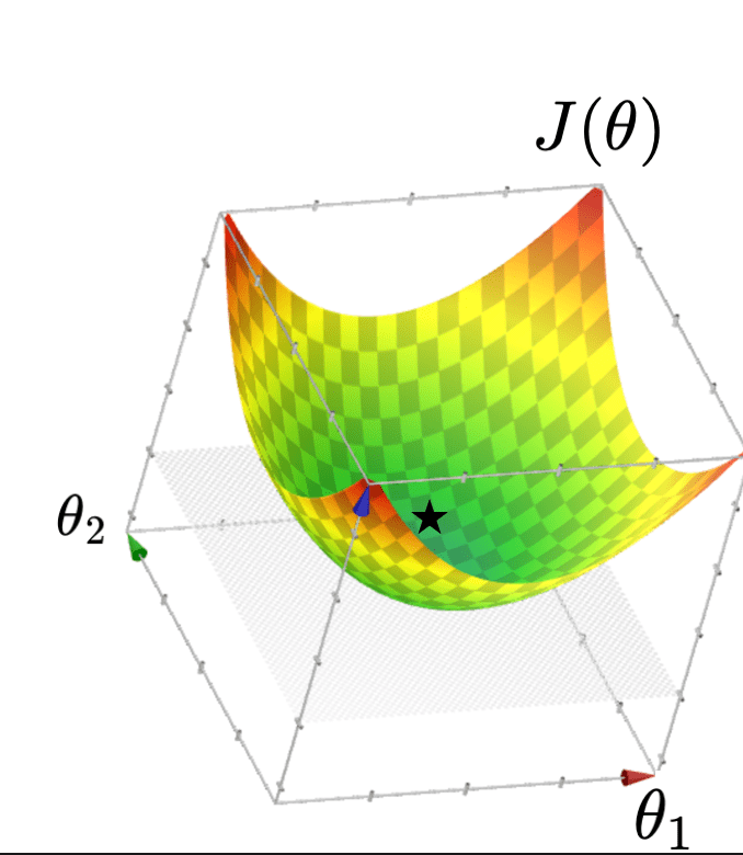
\( J(\theta) =\frac{1}{n}({X} \theta-{Y})^{\top}({X} \theta-{Y})\)
Let
Then
\(\in \mathbb{R}^{n\times d}\)
\(\in \mathbb{R}^{n\times 1}\)
\(\in \mathbb{R}^{d\times 1}\)
\(\in \mathbb{R}^{1\times 1}\)
X^\top X \in \mathbb{R}^{d \times d}
X^\top Y \in \mathbb{R}^{d \times 1}
By matrix calculus and optimization

\(\theta^*=\left({X}^{\top} {X}\right)^{-1} {X}^{\top} {Y}\)
Spotted in lab:
\(J(\theta) = (3 \theta-6)^{2}\)
1d-feature training data \((x,y) = (3,6)\)
\(X=x = [3]\)
\(Y=y = [6]\)
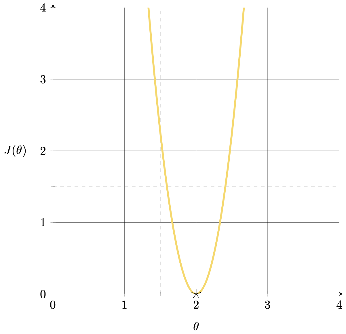
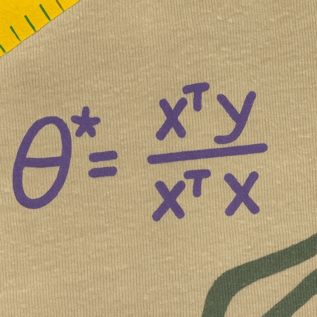
\(\theta^*=\left({X}^{\top} {X}\right)^{-1} {X}^{\top} {Y}\)
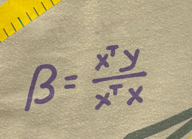
\(\theta^*=(xx)^{-1}(xy)\)
\(=\frac{xy}{xx} =\frac{y}{x} = \frac{6}{3}=2\)
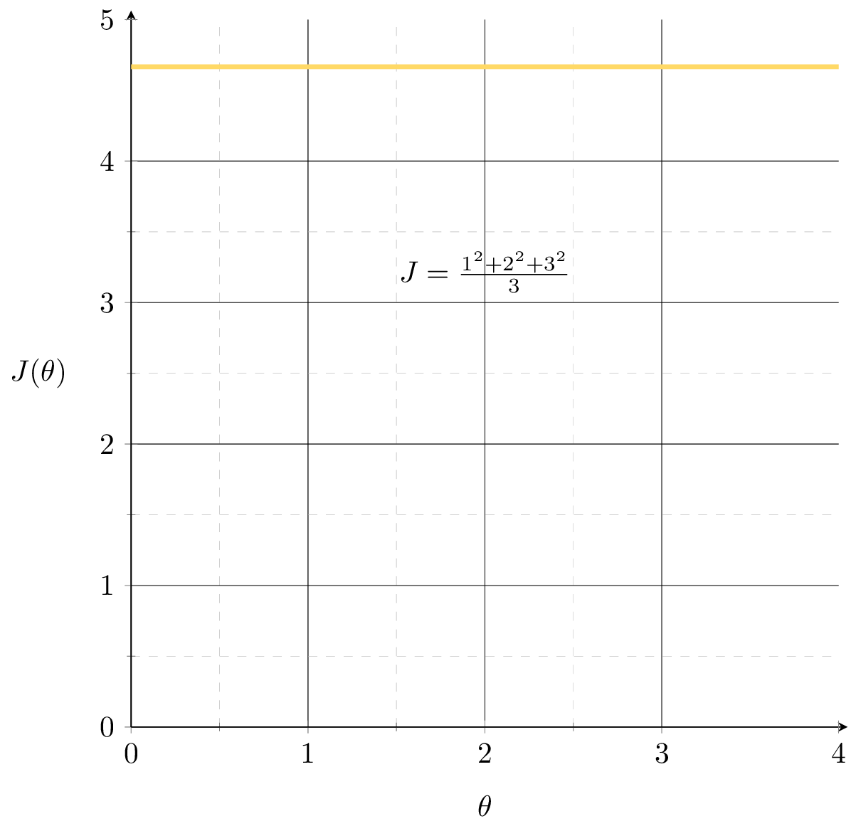
J(\theta) = \frac{1}{3}\left[(2 \theta-5)^2+\\(3 \theta-6)^{2}+(4 \theta-7)^2\right]
1-d feature training data set

| p1 | 2 | 5 |
| p2 | 3 | 6 |
| p3 | 4 | 7 |
x
y
\(X = \begin{bmatrix}2 \\3\\4\end{bmatrix}\)
\(Y = \begin{bmatrix}5 \\6 \\7\end{bmatrix}\)
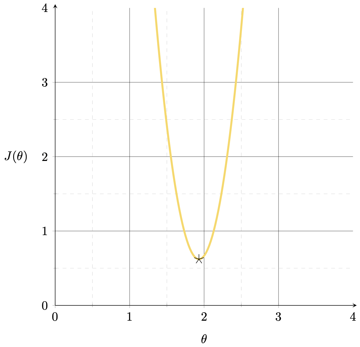
\(\theta^*=\left({X}^{\top} {X}\right)^{-1} {X}^{\top} {Y}\)
\(=\frac{X^{\top}Y}{X^{\top}X}= \frac{56}{29}\approx 1.93\)
\theta^{*}
= \bigl( [\,2 \; 3 \; 4\,] \begin{bmatrix}2 \\3\\4\end{bmatrix} \bigr)^{-1}
\;\; [\,2 \; 3 \; 4\,]
\begin{bmatrix}5 \\6 \\7\end{bmatrix}
Outline
- Recap: ordinary linear regression and the closed-form solution
-
The "trouble" with the closed-form solution
- mathematically, visually, practically
- Regularization, ridge regression, and hyperparameters
- Cross-validation
\(d=1\)
assume \(n=1\) and \(y=1\)
if the data is \((x,1) = (0.002,1)\)
if the data is \((x,y) = (-0.0002,1)\)
\(\theta^* = 500\)
\(\theta^* = -5,000\)
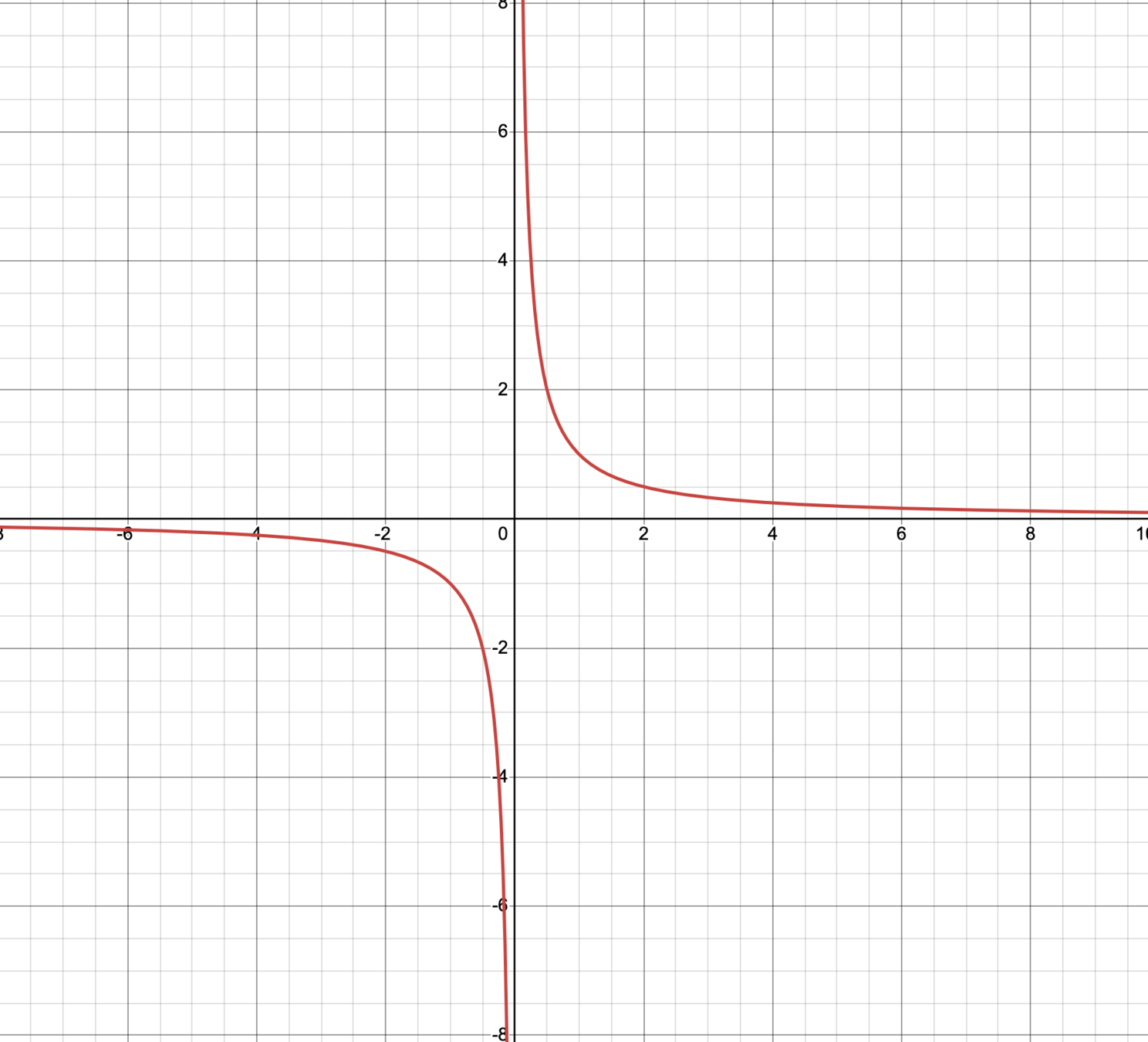
then \(\theta^*=\frac{1}{x}\)
most of the time, behaves nicely
\(\left({X}^{\top} {X}\right)\) is singular
\({X}\) is not full column rank
\(\left({X}^{\top} {X}\right)\) has zero eigenvalue(s)
\(\left({X}^{\top} {X}\right)\) is not full rank
the determinant of \(\left({X}^{\top} {X}\right)\) is zero
\Leftrightarrow
\Leftrightarrow
\Leftrightarrow
\Leftrightarrow
\(\theta^*=\left({X}^{\top} {X}\right)^{-1} {X}^{\top} {Y}\)
\(d\geq1\)
more generally,
most of the time, behaves nicely
but run into trouble when

if \({X}\) is not full column rank, then \(X^{\top}X\) is singular
- a. \(d=1\) and \(X \in \mathbb{R}^{n \times 1} \) is simply an all-zero vector, or
- b. \(n\)<\(d\), or
- c. columns (features) in \( {X} \) are linearly dependent.
X is not full column rank when:
all three cases have similar visual interpretations
(a). \(d=1\) and \(X \in \mathbb{R}^{n \times 1} \) is simply an all-zero vector
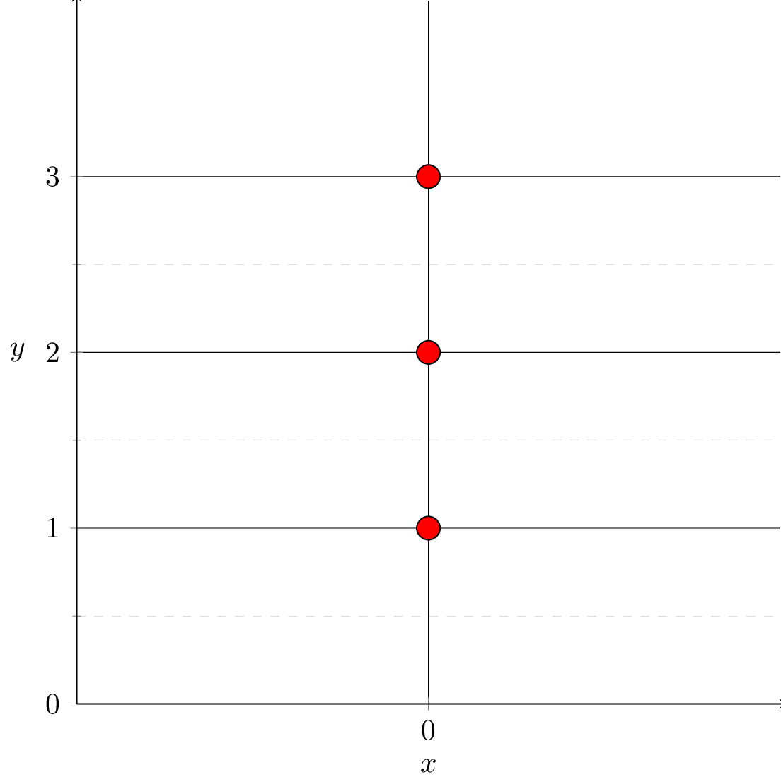
infinitely many optimal \(\theta\)
(b). \(n\)<\(d\)
infinitely many optimal \(\theta\)
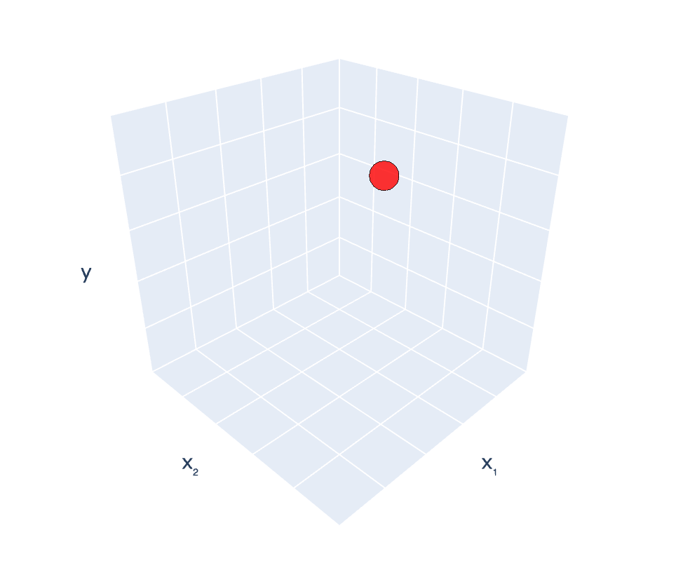
\((x_1, x_2) = (2,3), y =4\)
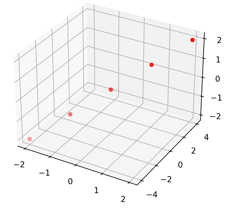
(c). columns (features) in \( {X} \) are linearly dependent.
infinitely many optimal \(\theta\)

\((x_1, x_2) = (2,3), y =7\)
\((x_1, x_2) = (4,6), y =8\)
\((x_1, x_2) = (6,9), y =9\)
infinitely many optimal \(\theta^*\)
temperature \(x_1\)
population \(x_2\)
energy used
\(y\)
temperature ( °F) \(x_1\)
temperature (°C) \(x_2\)
energy used
\(y\)
data
MSE
\(\theta^*=\left({X}^{\top} {X}\right)^{-1} {X}^{\top} {Y}\) is not well-defined
Quick Summary:
- This 👉 formula is not well-defined
Typically, \(X\) is full column rank
🥺
🥰
- \(\theta^*=\left({X}^{\top} {X}\right)^{-1} {X}^{\top} {Y}\)
- \(J(\theta)\) "curves up" everywhere
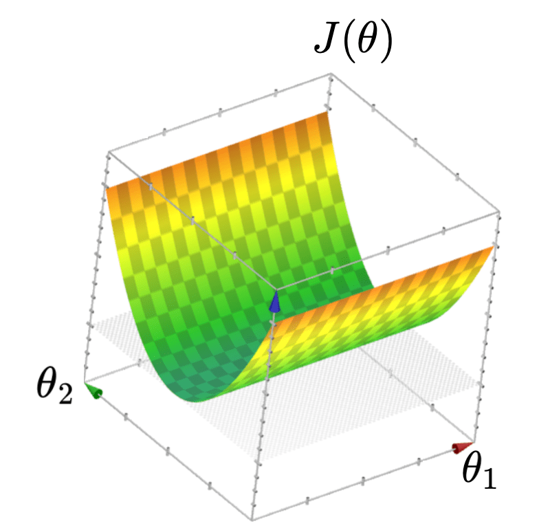
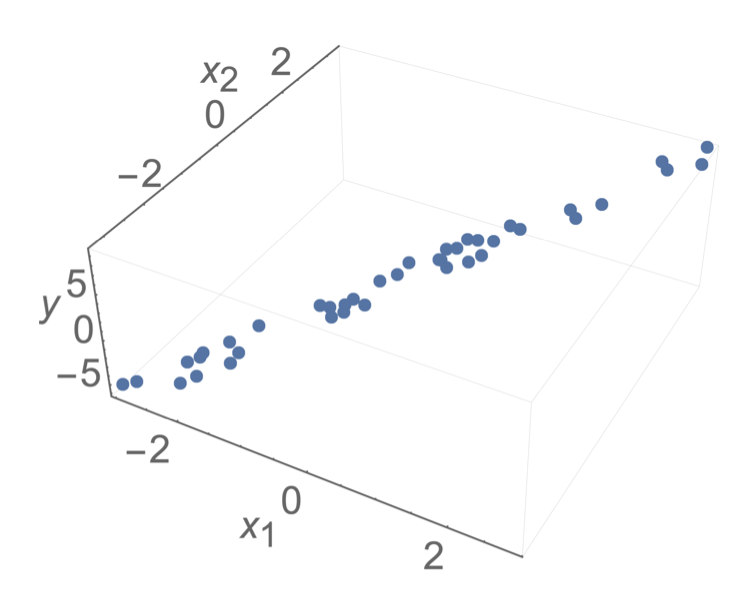
When \(X\) is not full column rank
- \(J(\theta)\) has a "flat" bottom, like a half pipe
- Infinitely many optimal hyperplanes
- \(\theta^*\) gives the unique optimal hyperplane
\(X^\top X\) becoming more invertible
formula isn't wrong, data is trouble-making
\(\theta^*=\left({X}^{\top} {X}\right)^{-1} {X}^{\top} {Y}\) does exist
\(\theta^*\) does give the unique optimal hyperplane
but
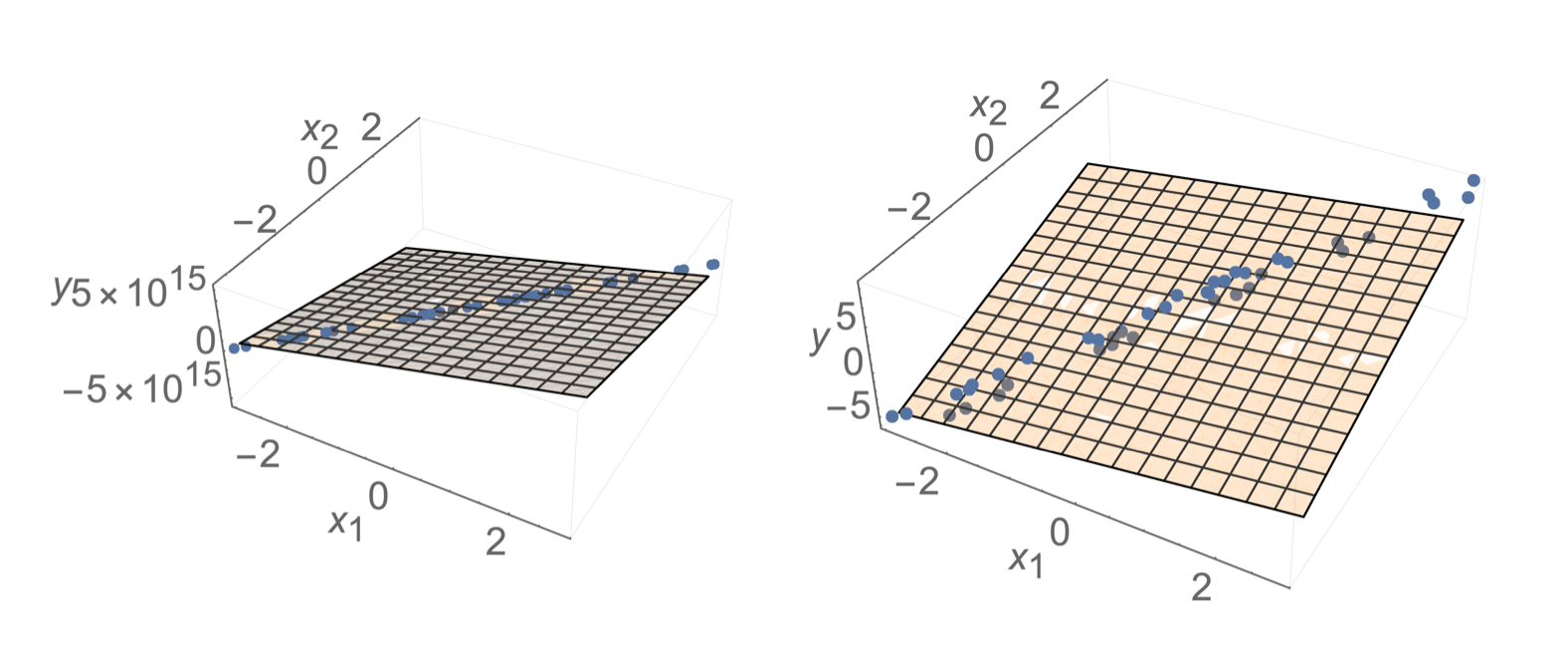
\(\theta^*\) tends to have huge magnitude
\(\theta^*\) tends to be very sensitive to the small changes in the data
\(\theta^*\) tends to overfit
when \(X^\top X\) is almost singular, technically
🥺
🥰
🥺
lots of hypotheses (lots of \(\theta\)s) fit the training data reasonably well
prefer \(\theta\) with small magnitude (less sensitive prediction when \(x\) changes slightly)
when \(X^\top X\) is almost singular
Outline
- Recap: ordinary linear regression and the closed-form solution
- The "trouble" with the closed-form solution
- mathematically, visually, practically
- Regularization, ridge regression, and hyperparameters
- Cross-validation
Regularization
- technique to combat overfitting
- at a high-level, it's to sacrifice some training performance, in the hope that testing behaves better
- many ways to regularize (e.g. implicit regularization, drop-out)
- we will look at a particularly simple regularization today, the so-called ridge or \(l2\)-regularization
Ridge Regression
- Add a squared penalty on the magnitude of the parameters
- \(J_{\text {ridge }}(\theta)=\frac{1}{n}({X} \theta-{Y})^{\top}({X} \theta-{Y})+\lambda\|\theta\|^2\)
- \(\lambda \) is a so-called "hyperparameter" (we've already seen a hyperparameter in lab 1)
- Setting \(\nabla_\theta J_{\text {ridge }}(\theta)=0\) we get \(\theta^*_{\text{ridge}}=\left({X}^{\top} {X}+n \lambda I\right)^{-1} {X}^{\top} {Y}\)
- \(\theta^*_{\text{ridge}}\) always exists, and is always the unique optimal parameter w.r.t. \(J_{\text {ridge }}\)
- (see ex/lab/hw for discussion about the offset.)
\((x_1, x_2) = (2,3), y =7\)
\((x_1, x_2) = (4,6), y =8\)
\((x_1, x_2) = (6,9), y =9\)
case (c) training data set again
Comments on \(\lambda\)
- chosen by users, before we even see the data
- controls the tradeoff between MSE and theta magnitude
- implicitly controls the "richness" of the hypothesis class
\boxed{h}
Regression
Algorithm
💻
\rightarrow
\downarrow
y
x
\downarrow
\(\in \mathbb{R}^d \)
\(\in \mathbb{R}\)
\(\mathcal{D}_\text{train}\)
\rightarrow
\(\left\{\left(x^{(1)}, y^{(1)}\right), \dots, \left(x^{(n)}, y^{(n)}\right)\right\}\)
hypothesis
🧠
- hypothesis class
- loss function
- hyperparameter
Outline
- Recap: ordinary linear regression and the closed-form solution
- The "trouble" with the closed-form solution
- mathematically, visually, practically
- Regularization, ridge regression, and hyperparameters
- Cross-validation
Validation
\boxed{h}
Regression
Algorithm
💻
\rightarrow
\(\mathcal{D}_\text{train}\)
\rightarrow
🧠 fixed
- hypothesis class
- loss function
- hyperparameter
\(\left\{\left(x^{(1)}, y^{(1)}\right), \dots, \left(x^{(n)}, y^{(n)}\right)\right\}\)
validation error
Cross-validation
\boxed{h}
Regression
Algorithm
💻
\rightarrow
\(\mathcal{D}_\text{train}\)
\rightarrow
🧠 fixed
- hypothesis class
- loss function
- hyperparameter
\(\left\{\left(x^{(1)}, y^{(1)}\right), \dots, \left(x^{(n)}, y^{(n)}\right)\right\}\)
chunk-1 validation error
\boxed{h}
Regression
Algorithm
💻
\rightarrow
\(\mathcal{D}_\text{train}\)
\rightarrow
🧠 fixed
- hypothesis class
- loss function
- hyperparameter
chunk-1 validation error
chunk-2 validation error
Cross-validation
\boxed{h}
Regression
Algorithm
💻
\rightarrow
\(\mathcal{D}_\text{train}\)
\rightarrow
🧠 fixed
- hypothesis class
- loss function
- hyperparameter
chunk-1 validation error
chunk-2 validation error
Cross-validation
...
chunk-\(k\) validation error
\left\{
\begin{array}{l}
\\
\\
\\
\\
\end{array}
\right.
averaging=>
cross-validation error
Comments on cross-validation
-
good idea to shuffle data first
-
a way to "reuse" data
-
cross-validation is more "reliable" than validation (less sensitive to chance)
-
it's not to evaluate a hypothesis (testing error is)
-
rather, it's to evaluate learning algorithm (e.g. hypothesis class choice, hyperparameter choice)
-
Can have an outer loop for picking good hyperparameter or hypothesis class
Summary
-
Closed-form formula for OLS is not well-defined when \(X^TX\) is singular, and we have infinitely many optimal \(\theta^*\).
-
Even in scenarios where \(X^TX\) is just ill-conditioned, we get sensitivity issues, many almost-as-good solutions, while the absolutely best \(\theta^*\) is overfitting to the data.
-
We need to indicate our preference somehow, and also fight overfitting.
-
Regularization helps battle overfitting -- by constructing a new optimization problem that implicitly prefers small-magnitude \(\theta.\)
-
Least-squares regularization leads to the ridge-regression formulation. (Good news: we can still solve it analytically!)
-
\(\lambda\) trades off training MSE and regularization strength, it's a hyperparameter.
-
Validation/cross-validation are a way to choose (regularization) hyperparameters.
Thanks!
We'd love to hear your thoughts.
\({X}\) is not full column rank
\(\left({X}^{\top} {X}\right)\) is not full rank
\Leftrightarrow
rank\((X) < d\)
rank\(({X}^{\top} {X}) < d\)
\Rightarrow
rank\(({AB})\leq\min\)[ rank\((A)\), rank\((B)\)]
for this (X^TX) matrix, since it's not just a genric, arbitrary matrix, we could read a bit more into it. it's square, symmetric
from the data's perspective
when is this (product) matrix singular?
\(X = \begin{bmatrix}x_1^{(1)} & \dots & x_d^{(1)}\\\vdots & \ddots & \vdots\\x_1^{(n)} & \dots & x_d^{(n)}\end{bmatrix}\)
feature 1
feature 2
\(X^\top X\)
each row is a data point
each column is a feature
6.390 IntroML (Fall25) - Lecture 2 Regularization and Cross-validation
By Shen Shen


