

Lecture 3: Gradient Descent Methods
Shen Shen
❤️ Feb 14, 2025 ❤️
11am, Room 10-250
Intro to Machine Learning

Outline
- Recap, motivation for gradient descent methods
- Gradient descent algorithm (GD)
- The gradient vector
- GD algorithm
- Gradient decent properties
- convex functions, local vs global min
- Stochastic gradient descent (SGD)
- SGD algorithm and setup
- GD vs SGD comparison
Outline
- Recap, motivation for gradient descent methods
- Gradient descent algorithm (GD)
- The gradient vector
- GD algorithm
- Gradient decent properties
- convex functions, local vs global min
- Stochastic gradient descent (SGD)
- SGD algorithm and setup
- GD vs SGD comparison
- This 👈 formula is not well-defined
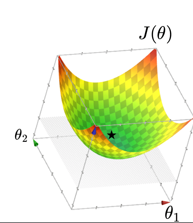
1. Typically, \(X\) is full column rank
🥺
🥰
- \(\theta^*=\left({X}^{\top} {X}\right)^{-1} {X}^{\top} {Y}\)
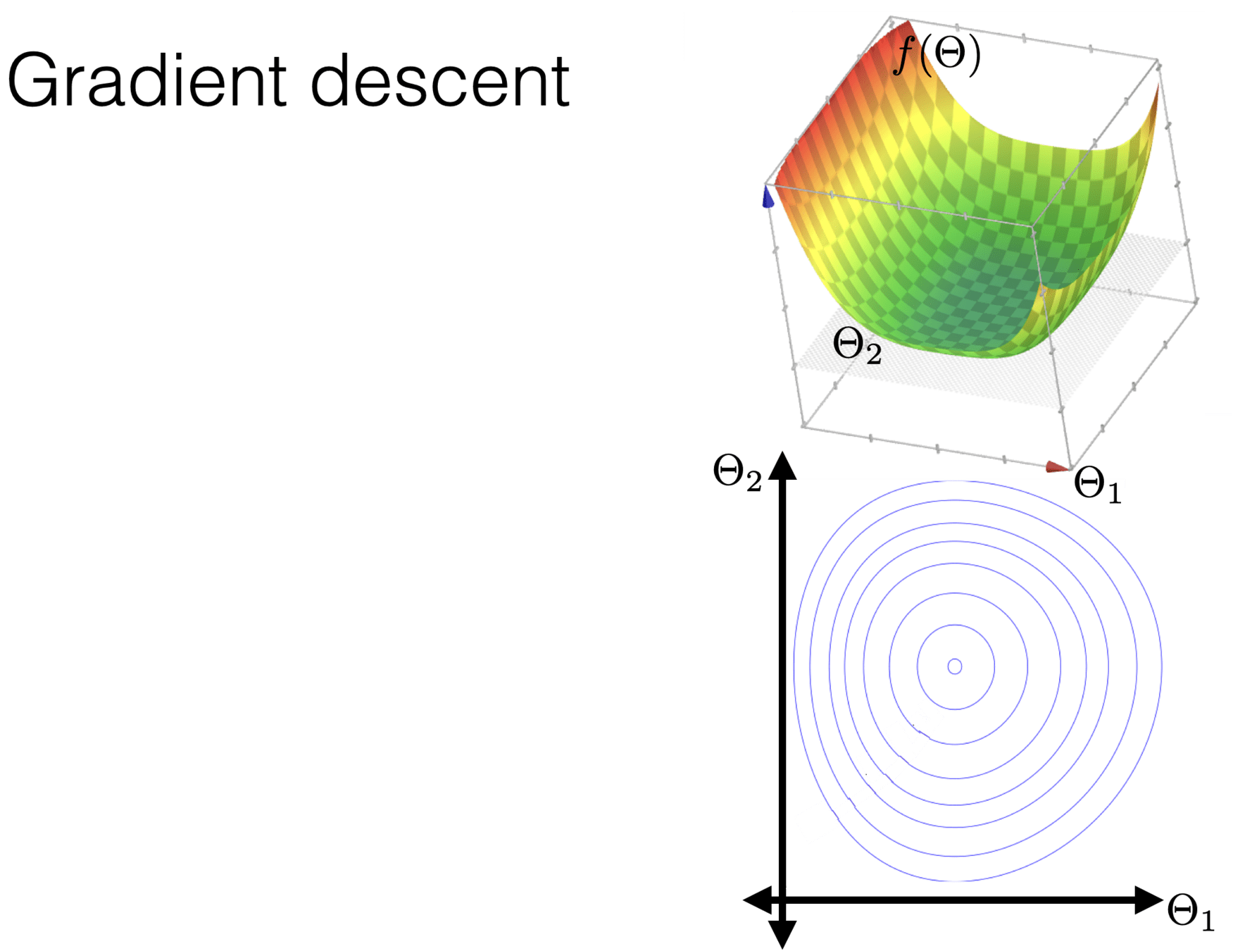
- \(J(\theta)\) looks like a bowl
a. either when \(n\)<\(d\) , or
b. columns (features) in \( {X} \) have linear dependency
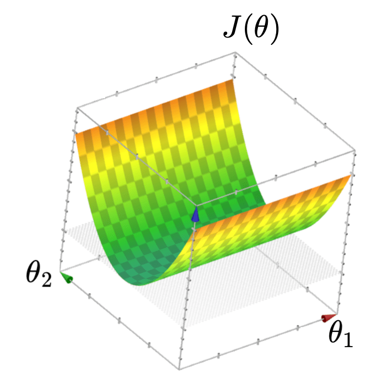
2. When \(X\) is not full column rank
- \(J(\theta)\) looks like a half-pipe
- Infinitely many optimal hyperplanes
- \(\theta^*\) gives the unique optimal hyperplane
Recall
- This 👈 formula is not well-defined
1. Typically, \(X\) is full column rank
🥺
- \(\theta^*=\left({X}^{\top} {X}\right)^{-1} {X}^{\top} {Y}\)
- \(J(\theta)\) looks like a bowl
2. When \(X\) is not full column rank
- \(J(\theta)\) looks like a half-pipe
- Infinitely many optimal hyperplanes
- \(\theta^*\) gives the unique optimal hyperplane
🥺
- \(\theta^*\) can be costly to compute (lab2, Q2.7)
- No way yet to obtain an optimal parameter
Want a more efficient and general method => gradient descent methods
🥰
Outline
- Recap, motivation for gradient descent methods
-
Gradient descent algorithm (GD)
- The gradient vector
- GD algorithm
- Gradient decent properties
- convex functions, local vs global min
- Stochastic gradient descent (SGD)
- SGD algorithm and setup
- GD vs SGD comparison
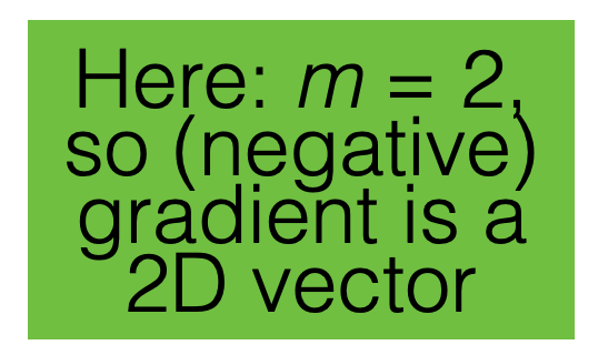
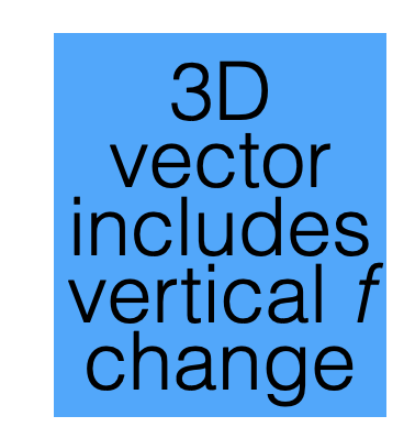
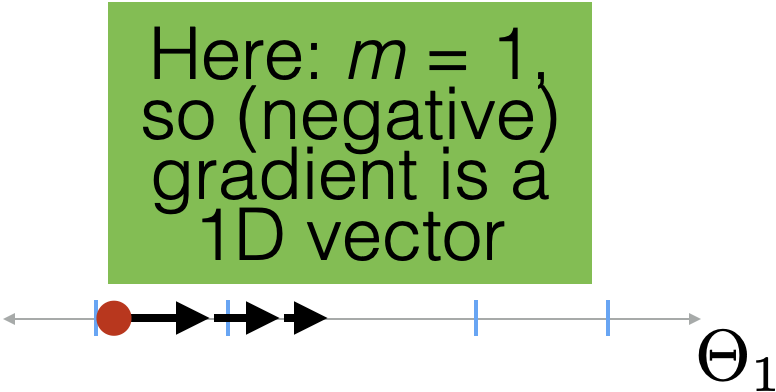
For \(f: \mathbb{R}^m \rightarrow \mathbb{R}\), its gradient \(\nabla f: \mathbb{R}^m \rightarrow \mathbb{R}^m\) is defined at the point \(p=\left(x_1, \ldots, x_m\right)\) as:
\nabla f(p)=\left[\begin{array}{c}
\frac{\partial f}{\partial x_1}(p) \\
\vdots \\
\frac{\partial f}{\partial x_m}(p)
\end{array}\right]
Sometimes the gradient is undefined or ill-behaved, but today it is well-behaved unless stated otherwise.
- The gradient generalizes the concept of a derivative to multiple dimensions.
- By construction, the gradient's dimensionality always matches the function input.
\nabla f(p)=\left[\begin{array}{c}
\frac{\partial f}{\partial x_1}(p) \\
\vdots \\
\frac{\partial f}{\partial x_m}(p)
\end{array}\right]
3. The gradient can be symbolic or numerical.
f(x, y, z) = x^2 + y^3 + z
example:
its symbolic gradient:
just like a derivative can be a function or a number.
evaluating the symbolic gradient at a point gives a numerical gradient:
\nabla f(x, y, z) = \begin{bmatrix}
2x \\
3y^2 \\
1
\end{bmatrix}
\nabla f(3, 2, 1) = \nabla f(x,y,z)\Big|_{(x,y,z)=(3,2,1)} = \begin{bmatrix}6\\12\\1\end{bmatrix}
4. The gradient points in the direction of the (steepest) increase in the function value.
\(\frac{d}{dx} \cos(x) \bigg|_{x = -4} = -\sin(-4) \approx -0.7568\)
\(\frac{d}{dx} \cos(x) \bigg|_{x = 5} = -\sin(5) \approx 0.9589\)
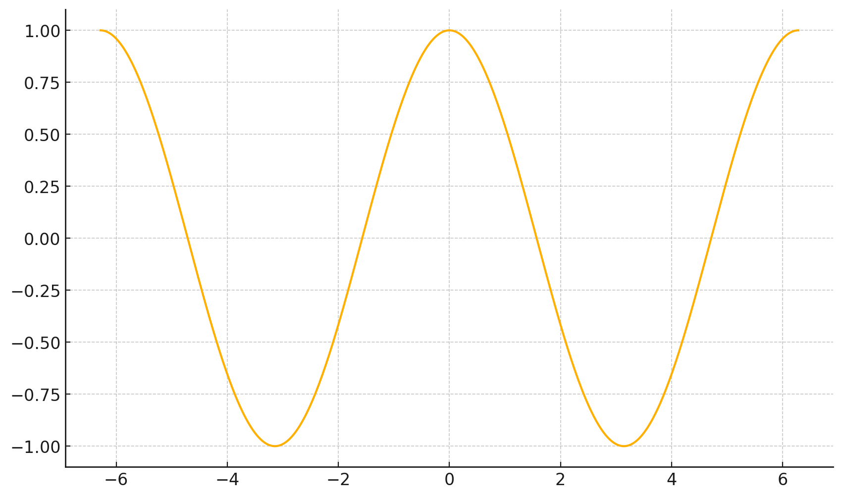
f(x)=\cos(x)
x
Outline
- Recap, motivation for gradient descent methods
-
Gradient descent algorithm (GD)
- The gradient vector
- GD algorithm
- Gradient decent properties
- convex functions, local vs global min
- Stochastic gradient descent (SGD)
- SGD algorithm and setup
- GD vs SGD comparison
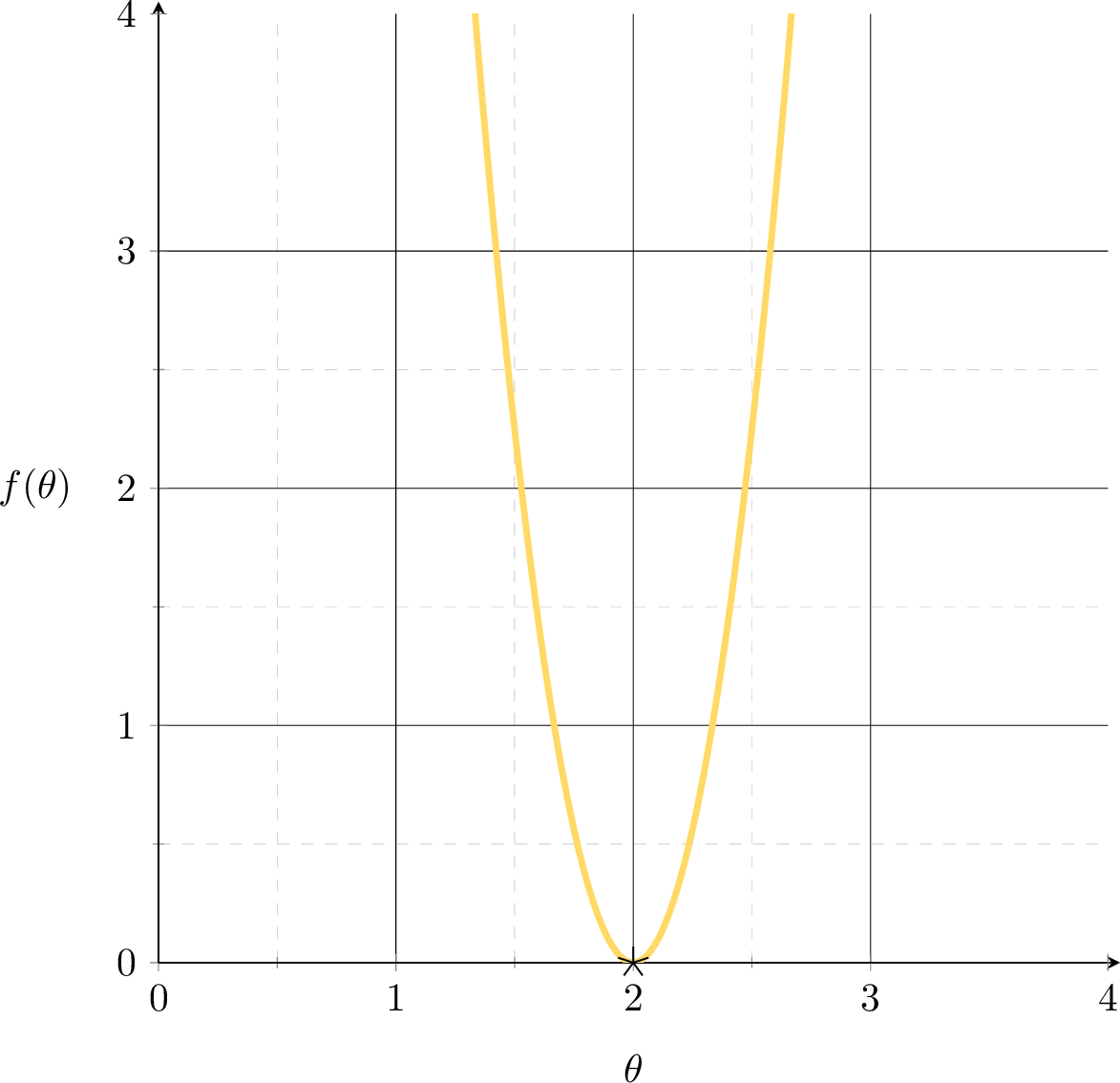
Want to fit a line (without offset) to minimize the MSE: \(f(\theta) = (3 \theta-6)^{2}\)
A single training data point
\((x,y) = (3,6)\)
MSE could get better.
How to formalize this?
Suppose we fit a line \(y= 1.5x\)
\(\nabla_\theta f = f'(\theta) \)
\(f(\theta) = (3 \theta-6)^{2}\)
\( = 2[3(3 \theta-6)]|_{\theta=1.5}\)
\(<0\)
MSE could get better. How to?
Leveraging the gradient.
Suppose we fit a line \(y= 1.5x\)
\(\nabla_\theta f = f'(\theta) \)
\(f(\theta) = (3 \theta-6)^{2}\)
\( = 2[3(3 \theta-6)]|_{\theta=2.4}\)
\(>0\)
MSE could get better. How to?
Leveraging the gradient.
Suppose we fit a line \(y= 2.4 x\)
hyperparameters
initial guess
of parameters
learning rate,
aka, step size
precision
1
2
3
4
5
6
7
8
1
2
3
4
5
6
7
8
level set

1
2
3
4
5
6
7
8


1
2
3
4
5
6
7
8
1
2
3
4
5
6
7
8
1
2
3
4
5
6
7
8
1
2
3
4
5
6
7
8
1
2
3
4
5
6
7
8

1
2
3
4
5
6
7
8
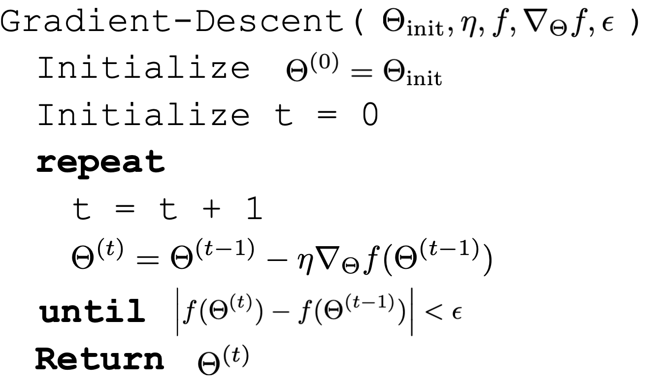
Q: what does this condition imply?
A: the gradient (at the current parameter nearly) is zero.
1
2
3
4
5
6
7
8
Other possible stopping criteria for line 7:
- Small parameter change: \( \|\Theta^{(t)} - \Theta^{(t-1)}\| < \epsilon \), or
- Small gradient norm: \( \|\nabla_{\Theta} f(\Theta^{(t)})\| < \epsilon \) also imply the same "gradient close to zero"
Outline
- Recap, motivation for gradient descent methods
-
Gradient descent algorithm (GD)
- The gradient vector
- GD algorithm
-
Gradient decent properties
- convex functions, local vs global min
- Stochastic gradient descent (SGD)
- SGD algorithm and setup
- GD vs SGD comparison

When minimizing a function, we aim for a global minimizer.


At a global minimizer
the gradient vector is the zero
\(\Rightarrow\)
\(\nLeftarrow\)

gradient descent can achieve this (to arbitrary precision)
the gradient vector is the zero
\(\Leftarrow\)
the objective function is convex
\{
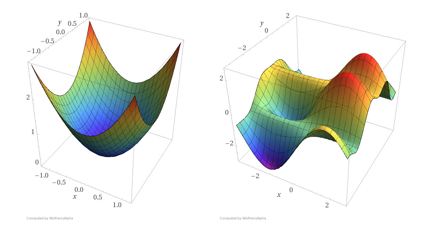
A function \(f\) is convex if any line segment connecting two points of the graph of \(f\) lies above or on the graph.
- \(f\) is concave if \(-f\) is convex.
- one can say a lot about optimization convergence for convex functions.
When minimizing a function, we aim for a global minimizer.
At a global minimizer
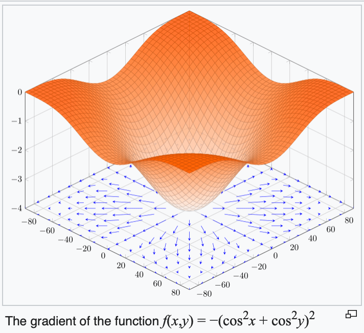
Some examples
Convex functions
Non-convex functions


- Assumptions:
- \(f\) is sufficiently "smooth"
- \(f\) is convex
- \(f\) has at least one global minimum
- Run gradient descent for sufficient iterations
- \(\eta\) is sufficiently small
- Conclusion:
- Gradient descent converges arbitrarily close to a global minimum of \(f\).
Gradient Descent Performance
if violated, may not have gradient,
can't run gradient descent
Gradient Descent Performance
- Assumptions:
- \(f\) is sufficiently "smooth"
- \(f\) is convex
- \(f\) has at least one global minimum
- Run gradient descent for sufficient iterations
- \(\eta\) is sufficiently small
- Conclusion:
- Gradient descent converges arbitrarily close to a global minimum of \(f\).
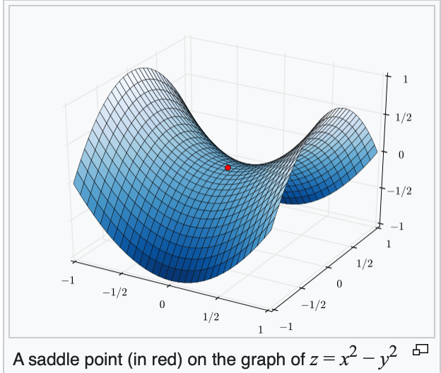
if violated, may get stuck at a saddle point
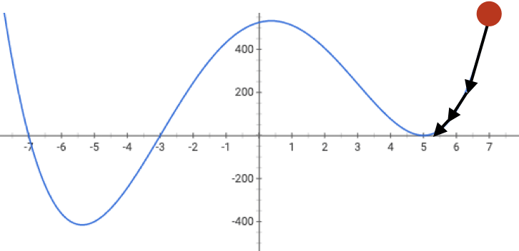
or a local minimum
- Assumptions:
- \(f\) is sufficiently "smooth"
- \(f\) is convex
- \(f\) has at least one global minimum
- Run gradient descent for sufficient iterations
- \(\eta\) is sufficiently small
- Conclusion:
- Gradient descent converges arbitrarily close to a global minimum of \(f\).
Gradient Descent Performance
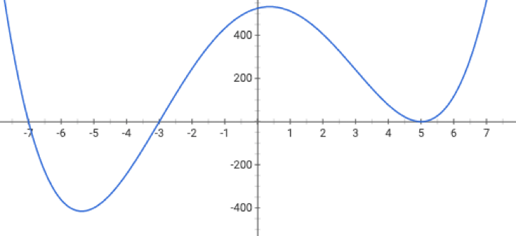
if violated:
may not terminate/no minimum to converge to

Gradient Descent Performance
- Assumptions:
- \(f\) is sufficiently "smooth"
- \(f\) is convex
- \(f\) has at least one global minimum
- Run gradient descent for sufficient iterations
- \(\eta\) is sufficiently small
- Conclusion:
- Gradient descent converges arbitrarily close to a global minimum of \(f\).
Gradient Descent Performance
- Assumptions:
- \(f\) is sufficiently "smooth"
- \(f\) is convex
- \(f\) has at least one global minimum
- Run gradient descent for sufficient iterations
- \(\eta\) is sufficiently small
- Conclusion:
- Gradient descent converges arbitrarily close to a global minimum of \(f\).
if violated:
see demo on next slide, also lab/recitation/hw
Outline
- Recap, motivation for gradient descent methods
- Gradient descent algorithm (GD)
- The gradient vector
- GD algorithm
- Gradient decent properties
- convex functions, local vs global min
-
Stochastic gradient descent (SGD)
- SGD algorithm and setup
- GD vs SGD comparison
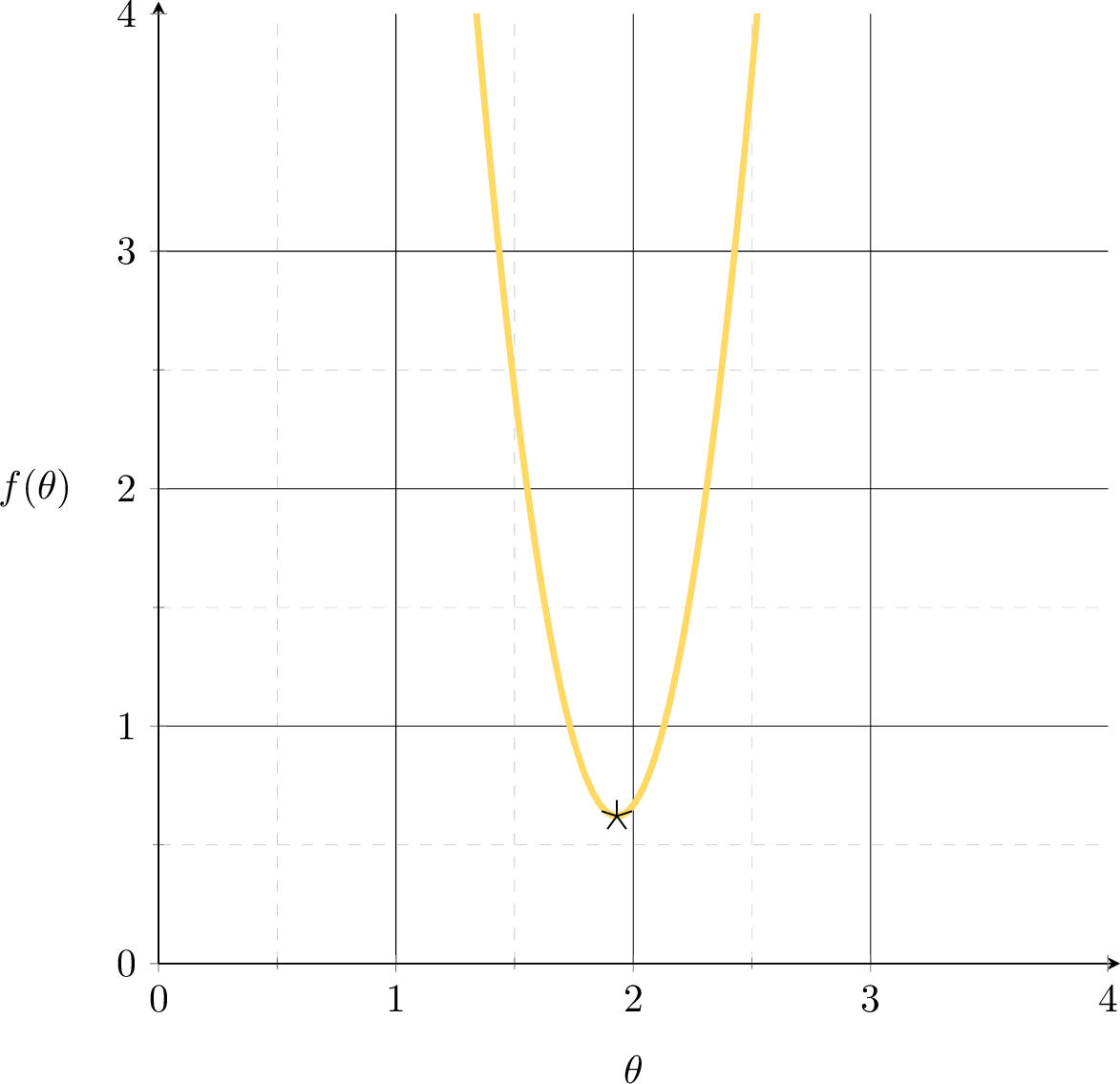
Fit a line (without offset) to the dataset, the MSE:
f(\theta) = \frac{1}{3}\left[(2 \theta-5)^2+(3 \theta-6)^{2}+(4 \theta-7)^2\right]
training data

| p1 | 2 | 5 |
| p2 | 3 | 6 |
| p3 | 4 | 7 |
x
y
Suppose we fit a line \(y= 2.5x\)
\(f(\theta) = \frac{1}{3}\left[(2 \theta-5)^2+(3 \theta-6)^{2}+(4 \theta-7)^2\right]\)
\(\nabla_\theta f = \frac{2}{3}[2(2 \theta-5)+3(3 \theta-6)+4(4 \theta-7)]\)
gradient can help MSE get better
\(f(\theta) = \frac{1}{3}\left[(2 \theta-5)^2+(3 \theta-6)^{2}+(4 \theta-7)^2\right]\)
\(\nabla_\theta f = \frac{2}{3}[2(2 \theta-5)+3(3 \theta-6)+4(4 \theta-7)]\)
- the MSE of a linear hypothesis:
- and its gradient w.r.t. \(\theta\):
| p1 | 2 | 5 |
| p2 | 3 | 6 |
| p3 | 4 | 7 |
x
y
\(f(\theta) = \frac{1}{3}\left[(2 \theta-5)^2+(3 \theta-6)^{2}+(4 \theta-7)^2\right]\)
- the MSE of a linear hypothesis:
| p1 | 2 | 5 |
| p2 | 3 | 6 |
| p3 | 4 | 7 |
x
y
\(\nabla_\theta f = \frac{2}{3}[2(2 \theta-5)+3(3 \theta-6)+4(4 \theta-7)]\)
- and its gradient w.r.t. \(\theta\):
Gradient of an ML objective
- the MSE of a linear hypothesis:
- and its gradient w.r.t. \(\theta\):
Using our example data set,
\(f(\theta) = \frac{1}{3}\left[(2 \theta-5)^2+(3 \theta-6)^{2}+(4 \theta-7)^2\right]\)
- the MSE of a linear hypothesis:
\(\nabla_\theta f = \frac{2}{3}[2(2 \theta-5)+3(3 \theta-6)+4(4 \theta-7)]\)
- and its gradient w.r.t. \(\theta\):
Using any dataset,
\nabla f(\theta) = \frac{2}{n} \sum_{i=1}^n\left(\theta^{\top} x^{(i)}-y^{(i)}\right) x^{(i)}
f(\theta) = \frac{1}{n} \sum_{i=1}^n\left(\theta^{\top} x^{(i)}-y^{(i)}\right)^2
Gradient of an ML objective
- An ML objective function is a finite sum
- and its gradient w.r.t. \(\theta\):
\nabla f(\theta) = \nabla (\frac{1}{n} \sum_{i=1}^n f_i(\theta))
\nabla f(\theta) = \frac{2}{n} \sum_{i=1}^n\left(\theta^{\top} x^{(i)}-y^{(i)}\right) x^{(i)}
= \frac{1}{n} \sum_{i=1}^n \nabla f_i(\theta)
In general,
f(\theta) = \frac{1}{n} \sum_{i=1}^n\left(\theta^{\top} x^{(i)}-y^{(i)}\right)^2
f(\theta)=\frac{1}{n} \sum_{i=1}^n f_i(\theta)
👋 (gradient of the sum) = (sum of the gradient)
👆
- the MSE of a linear hypothesis:
- and its gradient w.r.t. \(\theta\):
Gradient of an ML objective
- An ML objective function is a finite sum
- and its gradient w.r.t. \(\theta\):
\nabla f(\theta) = \nabla (\frac{1}{n} \sum_{i=1}^n f_i(\theta))
= \frac{1}{n} \sum_{i=1}^n \nabla f_i(\theta)
In general,
f(\theta)=\frac{1}{n} \sum_{i=1}^n f_i(\theta)
each of these \(\nabla f_i(\theta) \in \mathbb{R}^{d}\)
need to add \(n\) of them
Costly!
Let's do stochastic gradient descent (on the board).
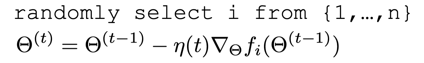
Stochastic gradient descent
\nabla f(\Theta)= \frac{1}{n} \sum_{i=1}^n \nabla f_i(\Theta)
\approx \nabla f_i(\Theta)
for a randomly picked data point \(i\)

Stochastic gradient descent performance
\(\sum_{t=1}^{\infty} \eta(t)=\infty\) and \(\sum_{t=1}^{\infty} \eta(t)^2<\infty\)
- Assumptions:
- \(f\) is sufficiently "smooth"
- \(f\) is convex
- \(f\) has at least one global minimum
- Run gradient descent for sufficient iterations
- \(\eta\) is sufficiently small and satisfies additional "scheduling" condition
- Conclusion:
- Stochastic gradient descent converges arbitrarily close to a global minimum of \(f\) with probability 1.
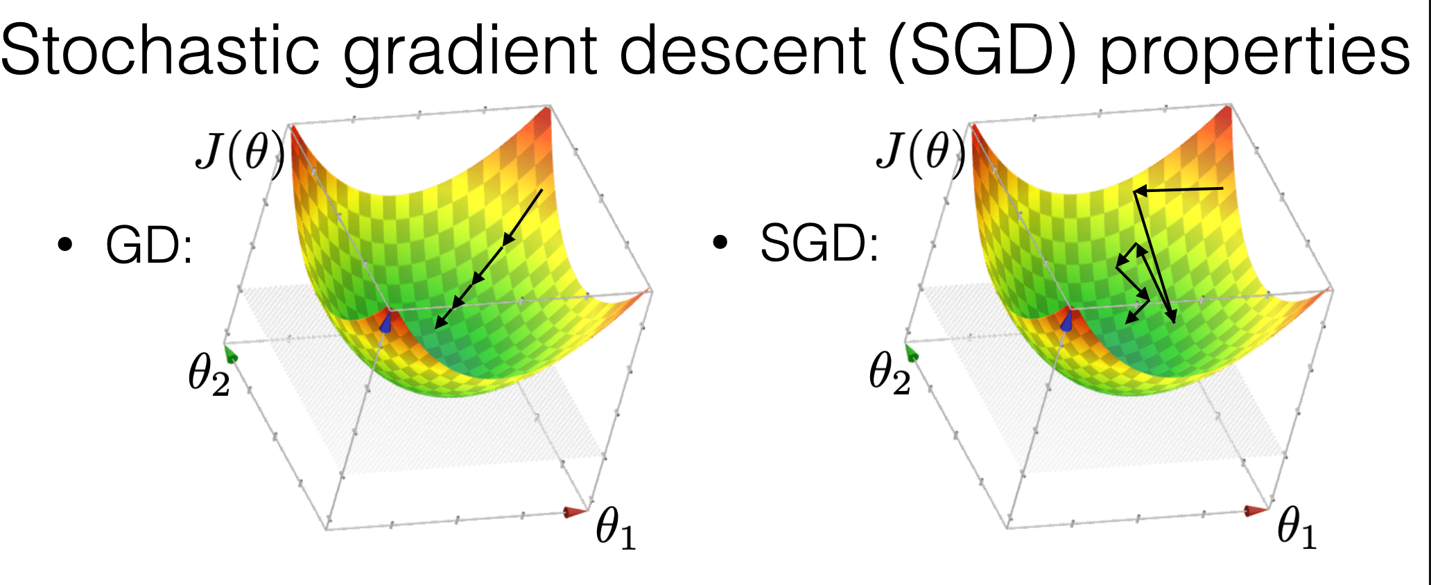
is more "random"
is more efficient
may get us out of a local min

Compared with GD, SGD
\nabla f(\Theta)= \frac{1}{n} \sum_{i=1}^n \nabla f_i(\Theta)
\approx \nabla f_i(\Theta)
Summary
-
Most ML methods can be formulated as optimization problems.
-
We won’t always be able to solve optimization problems analytically (in closed-form).
-
We won’t always be able to solve (for a global optimum) efficiently.
-
We can still use numerical algorithms to good effect. Lots of sophisticated ones available.
-
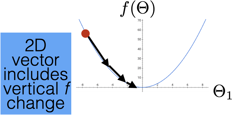
Introduce the idea of gradient descent in 1D: only two directions! But magnitude of step is important.
-
In higher dimensions the direction is very important as well as magnitude.
-
GD, under appropriate conditions (most notably, when objective function is convex), can guarantee convergence to a global minimum.
-
SGD: approximated GD, more efficient, more random, and less guarantees.
Thanks!
We'd love to hear your thoughts.
- A function \(f\) on \(\mathbb{R}^m\) is convex if any line segment connecting two points of the graph of \(f\) lies above or on the graph.
- For convex functions, all local minima are global minima.
What do we need to know:
- Intuitive understanding of the definition
- If given a function, can determine if it's convex. (We'll only ever give at most 2-dimensional input, these are "easy" cases where visual understanding suffices)
- Understand how gradient descent algorithms may fail without convexity.
- Recognize that OLS loss function is convex, ridge regression loss is (strictly) convex, and later cross-entropy loss function is convex too.
From lecture 2 feedback and questions:
1. post slides before lecture.
yes, will do.
2. what's the difference between notes and lectures.
same scope vs different media. think of novel versus movie. also one form might just fit your schedule better.
Oh should also mention the new WIP html notes. goal and seek suggestions
3. better mic positioning
yep will do.
6.390 IntroML (Spring25) - Lecture 3 Gradient Descent Methods
By Shen Shen


