
Lecture 1: Representation Learning
Shen Shen
March 31, 2025
2:30pm, Room 32-144
Modeling with Machine Learning for Computer Science
Course Staff

Shen Shen
Wed 4-5pm & Fri 2-3pm
24-328
Amit Schechter
Thursdays 1-3pm
45-324
Derek Lim
Tuesdays 3-5pm,
45-324
Course Staff
Amit Schechter
Thursdays 1-3pm
45-324
Derek Lim
Tuesdays 3-5pm,
45-324


Shen Shen
Wed 4-5pm & Fri 2-3pm
24-328
Course info/logistics
- This 6-unit course is designed to be paired with the broader co-requisite 6.C01/6.C51.
- We focus on “modeling with machine learning” for EECS-related topics and applications, and address the shared methodology, considerations, and challenges.
- There are other 6-unit modules you could take tailored to different departments.
Course Components and Grading
- Project: the course is project oriented (50% of the grade is from the project)
- form team, choose topic (not graded, but important! Due next Monday)
- how to (creatively) frame/formalize your task (10%)
- how to select/design your method (15%)
- how to evaluate/assess/interpret results (15%)
- communicating your findings via presentation (10%)
- Homeworks (30%): 4 weekly psets, each roughly 3 problems, graded best 2 out of 3 (grad version solve one required problem.)
- Exam (20%): in class, based on homeworks
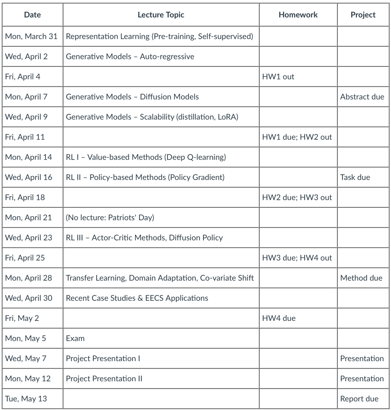
Semester at a glance
Generative AI
Reinforcement Learning
Integration
What is this focus on “modeling”?
- Example: we wish to realize a diagnostic helper for a physician
- Modeling is not: simply applying an off-the-shelf method to a problem (e.g., using a LLM to generate candidate diagnosis for a physician to consider in response to a patient description)
- Modeling is not: developing a new method to address a generic problem (e.g., improving transformer efficiency, making them dynamically configurable)
- Modeling is about relating methods and tasks (e.g., figuring out how that LLM can be made fair or robust, what fine-tuning data to use, how to incorporate physician feedback, etc)
Modeling with Machine Learning
- Frame the task/capability you are after
ask the right questions, formalize the problem as a learning to predict/control task - Solve (data + method + optimization)
select/tailor/design a machine learning method to solve the task with the given data; specify the hypothesis class, objective function, optimization algorithm - Assess/understand the results
interpret/analyze the results, whether the method worked/when it is likely to work
What are some typical EECS applications?
- Computer Vision
- Natural Language Understanding
- Robotics, Planning, & Control Systems
- Algorithmic Design
- Program Synthesis & Code Generation
- Scientific Computing & Numerical Methods
- Formal Verification & Theorem Proving
- Programming Languages & Bug Detection
- Chip & Hardware Design
\dots
layer
linear combo
activations
Recap:
\dots
\dots
layer
\dots
x_1
x_2
x_d
input
\Sigma
f(\cdot)
\Sigma
f(\cdot)
\Sigma
f(\cdot)
\Sigma
f(\cdot)
\Sigma
f(\cdot)
\Sigma
f(\cdot)
\Sigma
f(\cdot)
neuron
learnable weights
hidden
output
\sigma_1 = \sigma(5 x_1 -5 x_2 + 1)
\sigma_2 = \sigma(-5 x_1 + 5 x_2 + 1)
\(-3(\sigma_1 +\sigma_2)\)
recall this example
x_1
x_2
1
\Sigma
f(\cdot)
\Sigma
f(\cdot)
\Sigma
f(\cdot)
\(f =\sigma(\cdot)\)
\(f(\cdot) \) identity function
W^1
W^2
\sigma_1 = \sigma(5 x_1 -5 x_2 + 1)
\sigma_2 = \sigma(-5 x_1 + 5 x_2 + 1)
5
-5
1
-5
5
1
-3
-3
\(-3(\sigma_1 +\sigma_2)\)
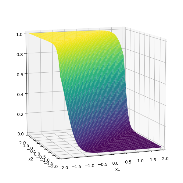
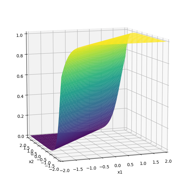
compositions of ReLU(s) can be quite expressive
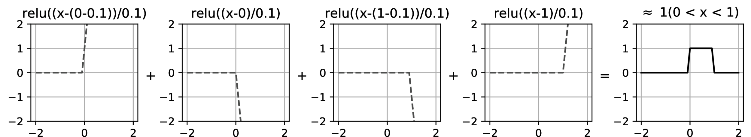
in fact, asymptotically, can approximate any function!
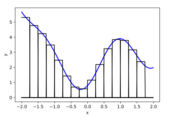
(image credit: Phillip Isola)
x^{(1)}
y^{(1)}
f^1
\begin{aligned}
& W^1 \\
\end{aligned}
\begin{aligned}
& W^2 \\
\end{aligned}
\begin{aligned}
& W^L \\
\end{aligned}
f^2
f^L
g^{(1)}
\(\dots\)
f^2\left(\hspace{2cm}; \mathbf{W}^2\right)
f^1(\mathbf{x}^{(i)}; \mathbf{W}^1)
f^L\left(\dots \hspace{3.5cm}; \dots \mathbf{W}^L\right)
Forward pass: evaluate, given the current parameters
- the model outputs \(g^{(i)}\) =
- the loss incurred on the current data \(\mathcal{L}(g^{(i)}, y^{(i)})\)
- the training error \(J = \frac{1}{n} \sum_{i=1}^{n}\mathcal{L}(g^{(i)}, y^{(i)})\)
\mathcal{L}(g^{(1)}, y^{(1)})
\mathcal{L}(g, y)
\mathcal{L}(g^{(n)}, y^{(n)})
\underbrace{\quad \quad \quad \quad \quad }
\dots
\dots
\dots
n
linear combination
loss function
(nonlinear) activation
x
\(\dots\)
y
f^1
\begin{aligned}
& W^1 \\
\end{aligned}
\begin{aligned}
& W^2 \\
\end{aligned}
\begin{aligned}
& W^L \\
\end{aligned}
f^2
f^L
\mathcal{L}(g,y)
g
Z^L
A^2
Z^2
A^1
Z^1
\frac{\partial \mathcal{L}(g,y)}{\partial g}
\frac{\partial g}{\partial Z^{L}}
\frac{\partial Z^3}{\partial A^{2}}\frac{\partial A^4}{\partial Z^{3}} \dots \frac{\partial Z^L}{\partial A^{L-1}}
\frac{\partial A^2}{\partial Z^{2}}
\frac{\partial \mathcal{L}(g,y)}{\partial Z^2}
\underbrace{\hspace{4cm}}
\underbrace{\hspace{4.7cm}}
\frac{\partial Z^2}{\partial W^{2}}
\frac{\partial \mathcal{L}(g,y)}{\partial W^2}
back propagation: reuse of computation
\underbrace{\hspace{6.5cm}}
\frac{\partial Z^2}{\partial A^{1}}
\frac{\partial A^1}{\partial Z^{1}}
\frac{\partial Z^1}{\partial W^{1}}
x
\(\dots\)
y
f^1
\begin{aligned}
& W^1 \\
\end{aligned}
\begin{aligned}
& W^2 \\
\end{aligned}
\begin{aligned}
& W^L \\
\end{aligned}
f^2
f^L
\mathcal{L}(g,y)
g
Z^L
A^2
Z^2
A^1
Z^1
\frac{\partial \mathcal{L}(g,y)}{\partial g}
\frac{\partial g}{\partial Z^{L}}
\frac{\partial Z^3}{\partial A^{2}}\frac{\partial A^4}{\partial Z^{3}} \dots \frac{\partial Z^L}{\partial A^{L-1}}
\frac{\partial A^2}{\partial Z^{2}}
\frac{\partial \mathcal{L}(g,y)}{\partial Z^2}
\underbrace{\hspace{4cm}}
\frac{\partial \mathcal{L}(g,y)}{\partial W^1}
\underbrace{\hspace{4.7cm}}
\frac{\partial Z^2}{\partial W^{2}}
\frac{\partial \mathcal{L}(g,y)}{\partial W^2}
back propagation: reuse of computation
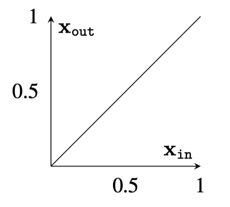
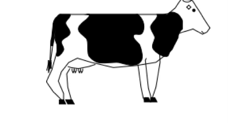
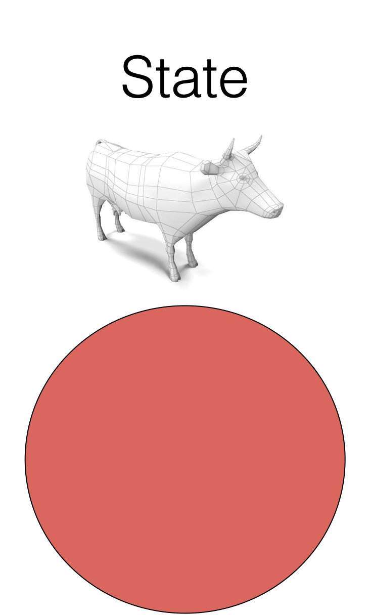
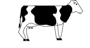
Two different ways to visualize a function
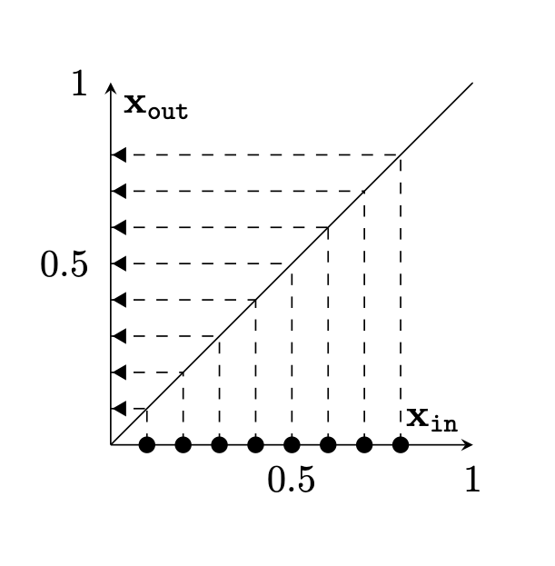
Two different ways to visualize a function
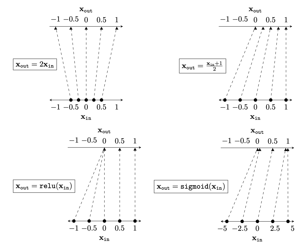
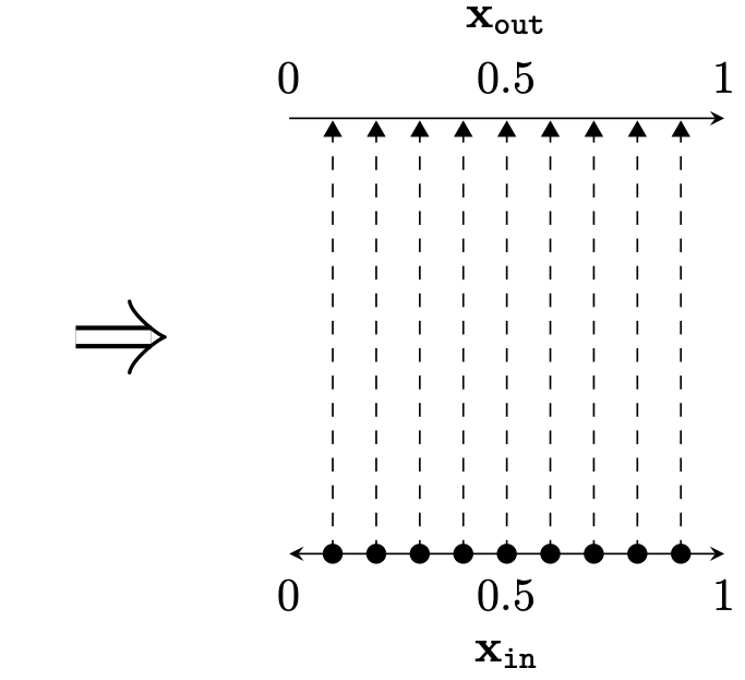
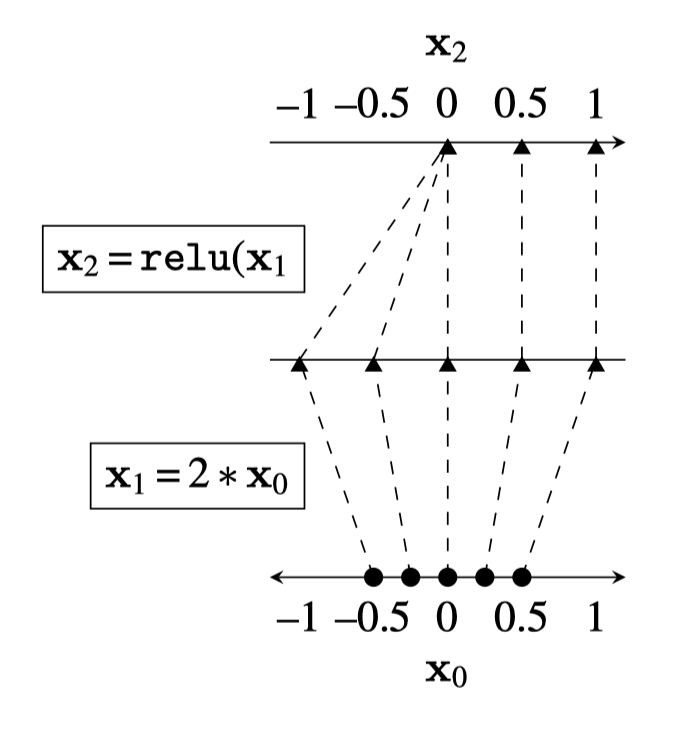
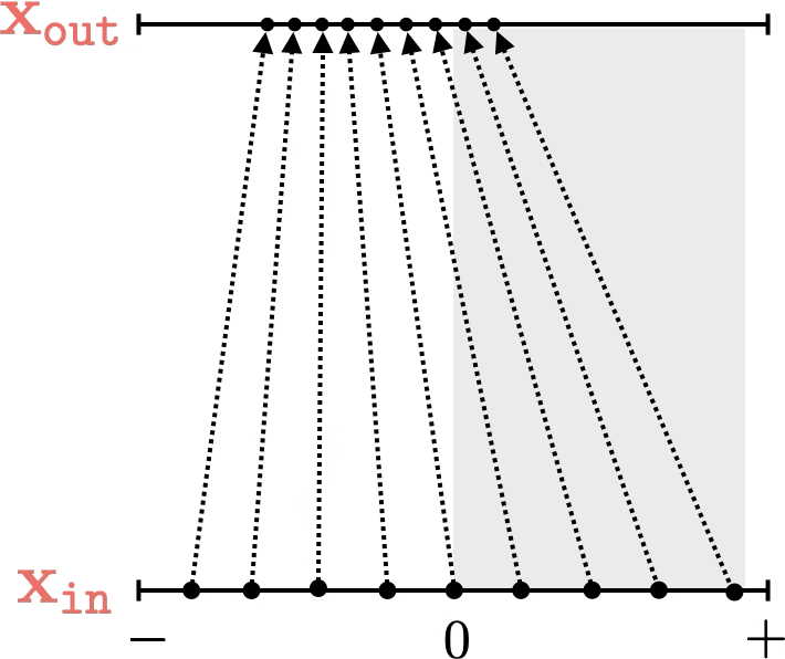
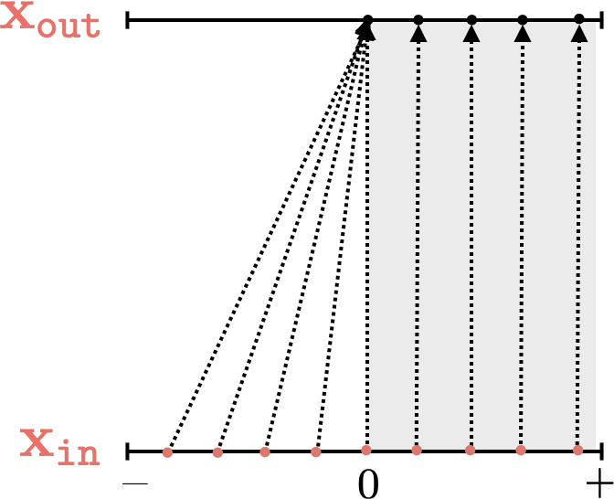
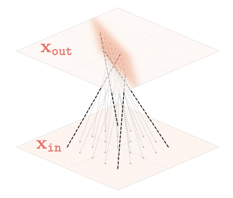
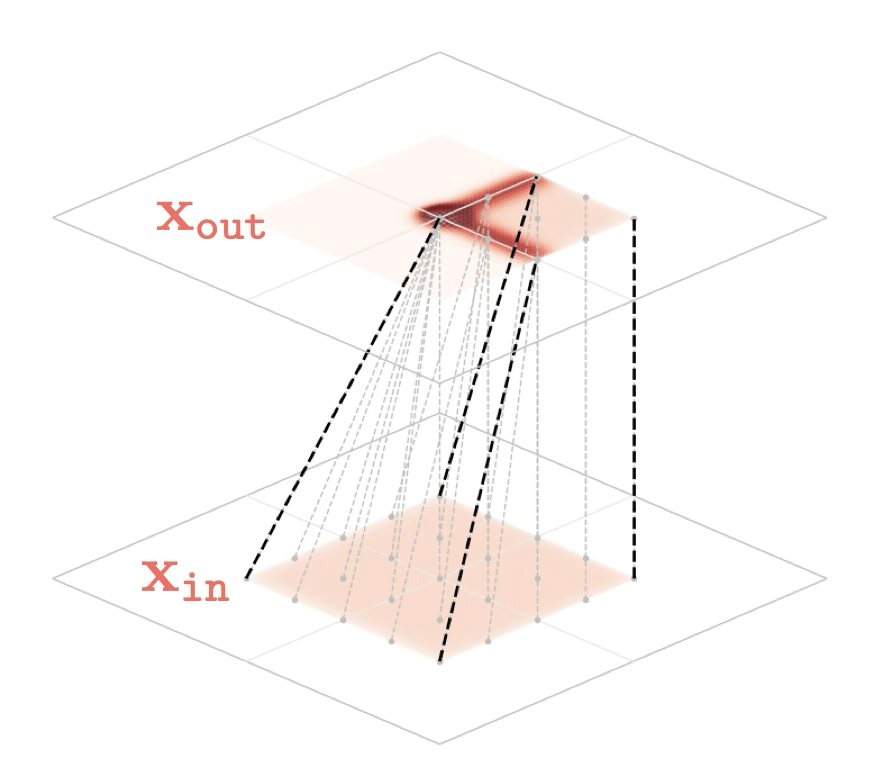
Representation transformations for a variety of neural net operations
and stack of neural net operations
)

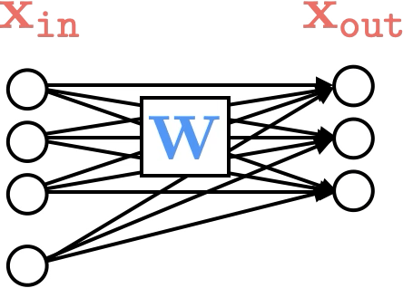
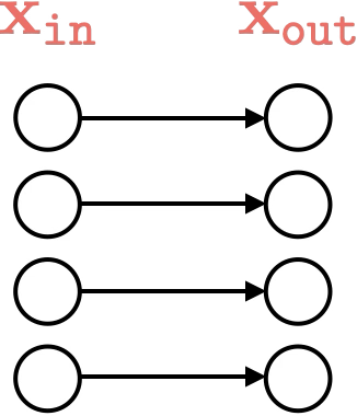
wiring graph
equation
mapping 1D
mapping 2D


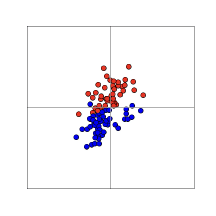
Training data
x
z_1
a_1
z_2
g
{z}_1=\text { linear }(x)
{a}_1=\text { ReLU}(z_1)
g=\text {softmax}(z_2)
{z}_2=\text { linear }(a_1)
x\in \mathbb{R^2}
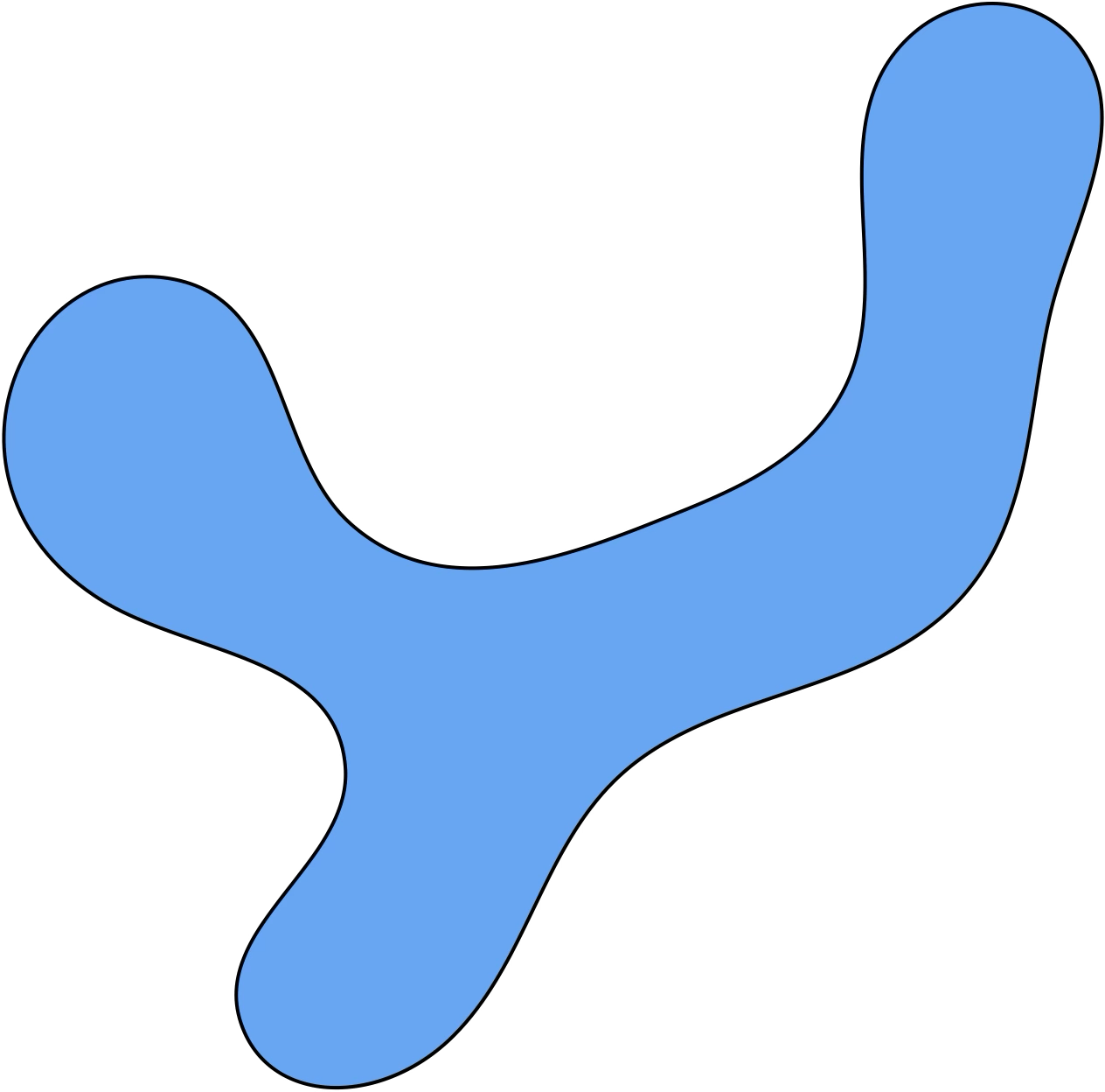

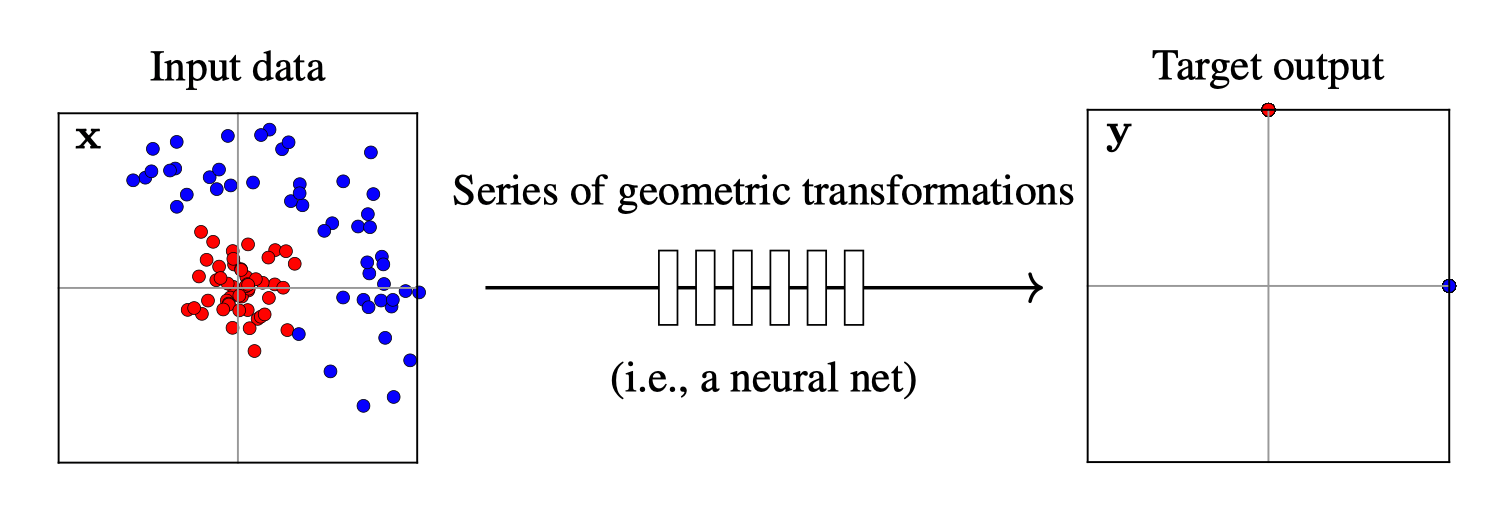
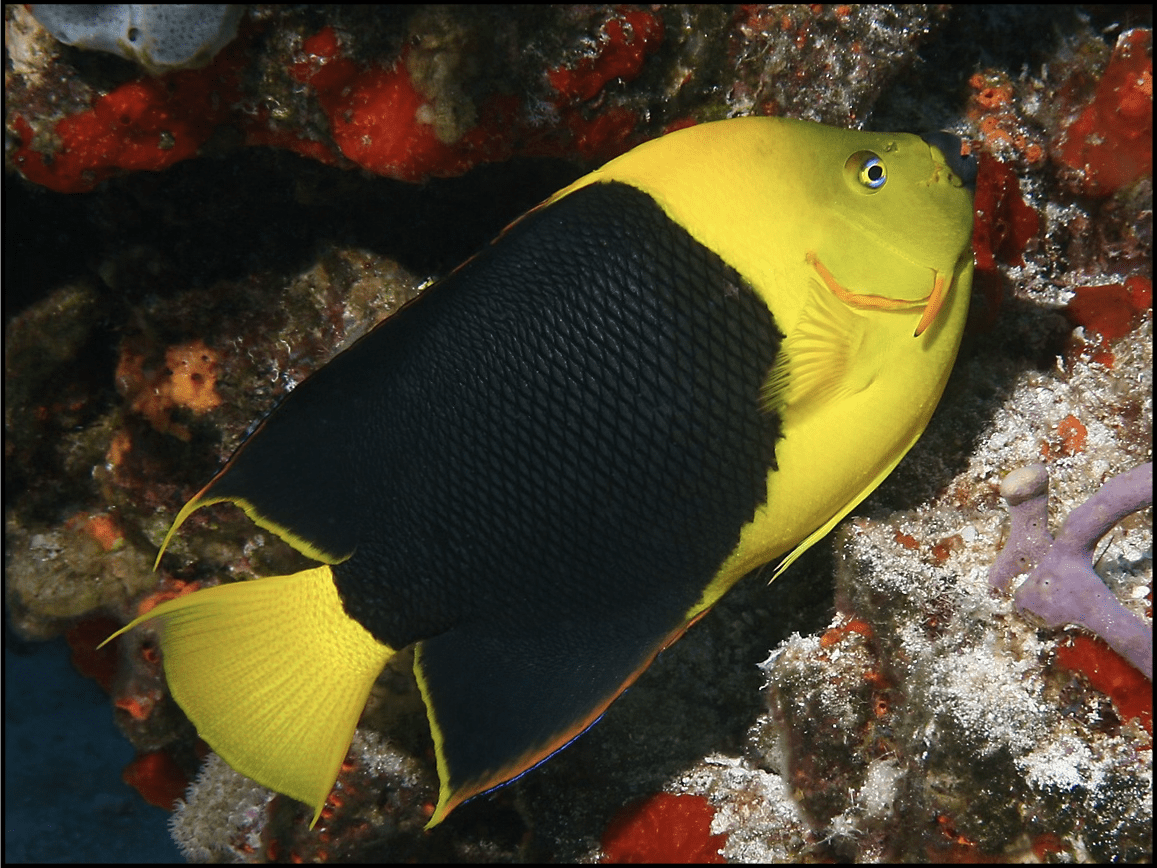
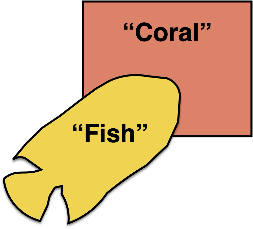
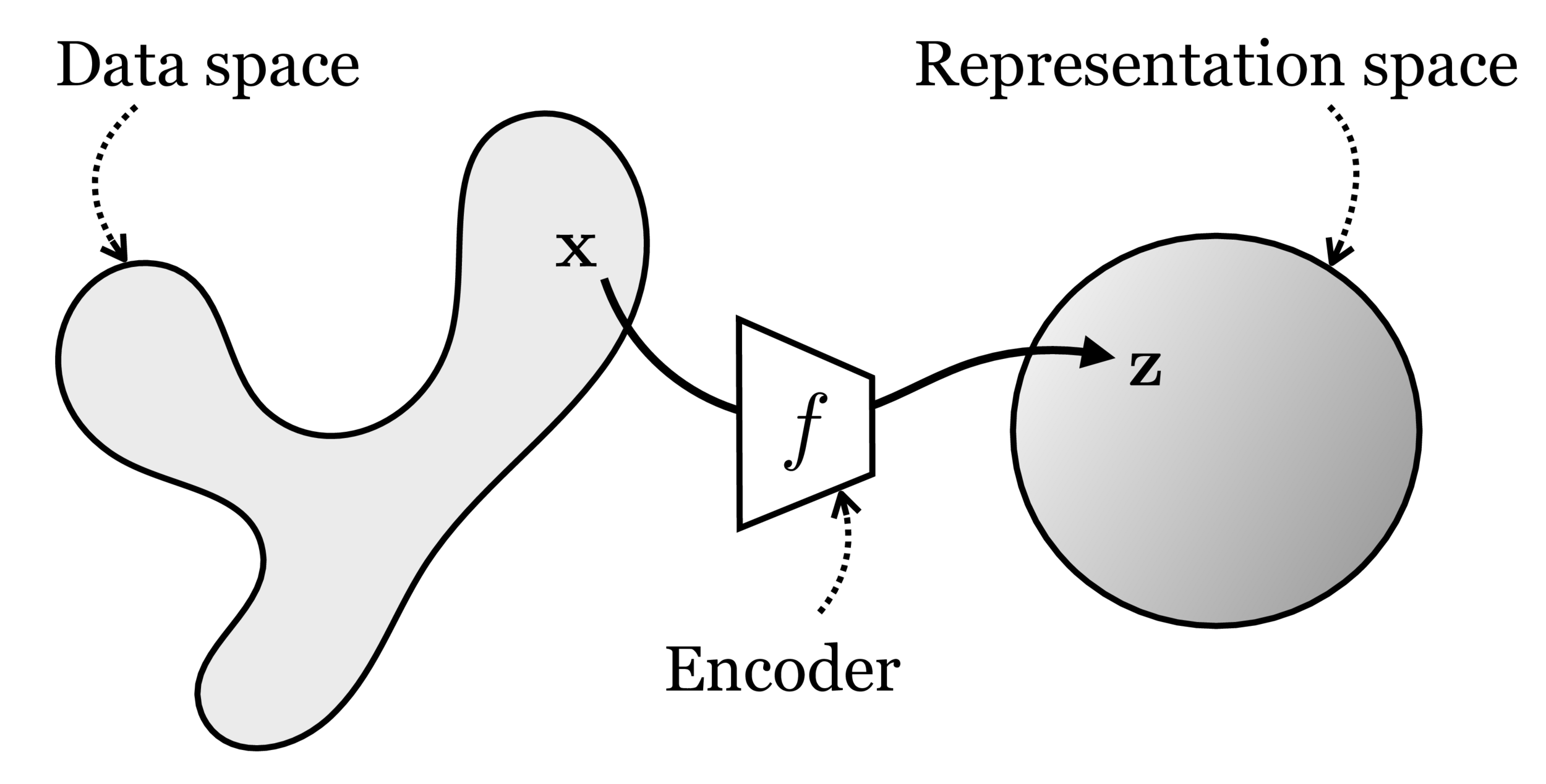
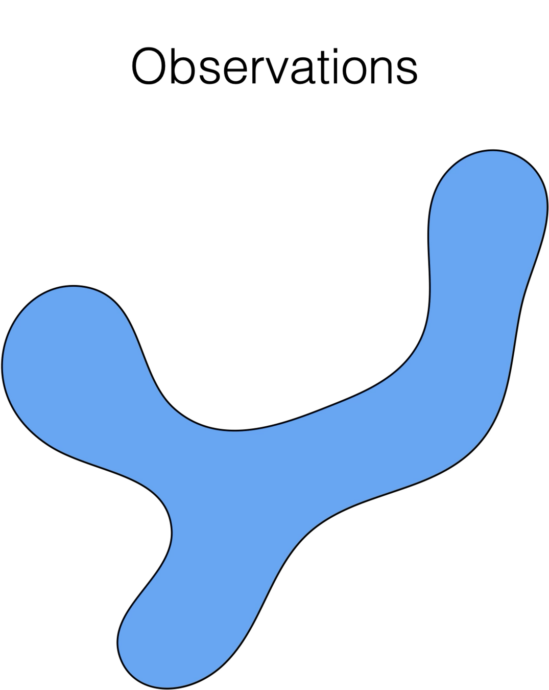
maps from complex data space to simple embedding space

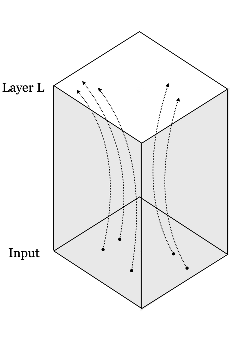
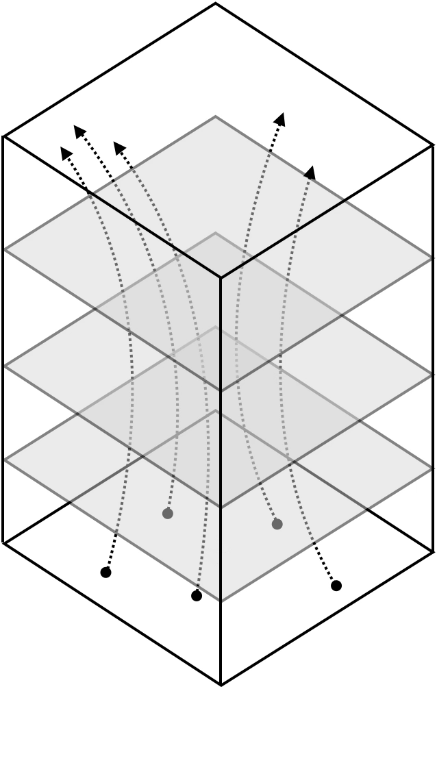
Neural networks are representation learners
Deep nets transform datapoints, layer by layer
Each layer gives a different representation (aka embedding) of the data
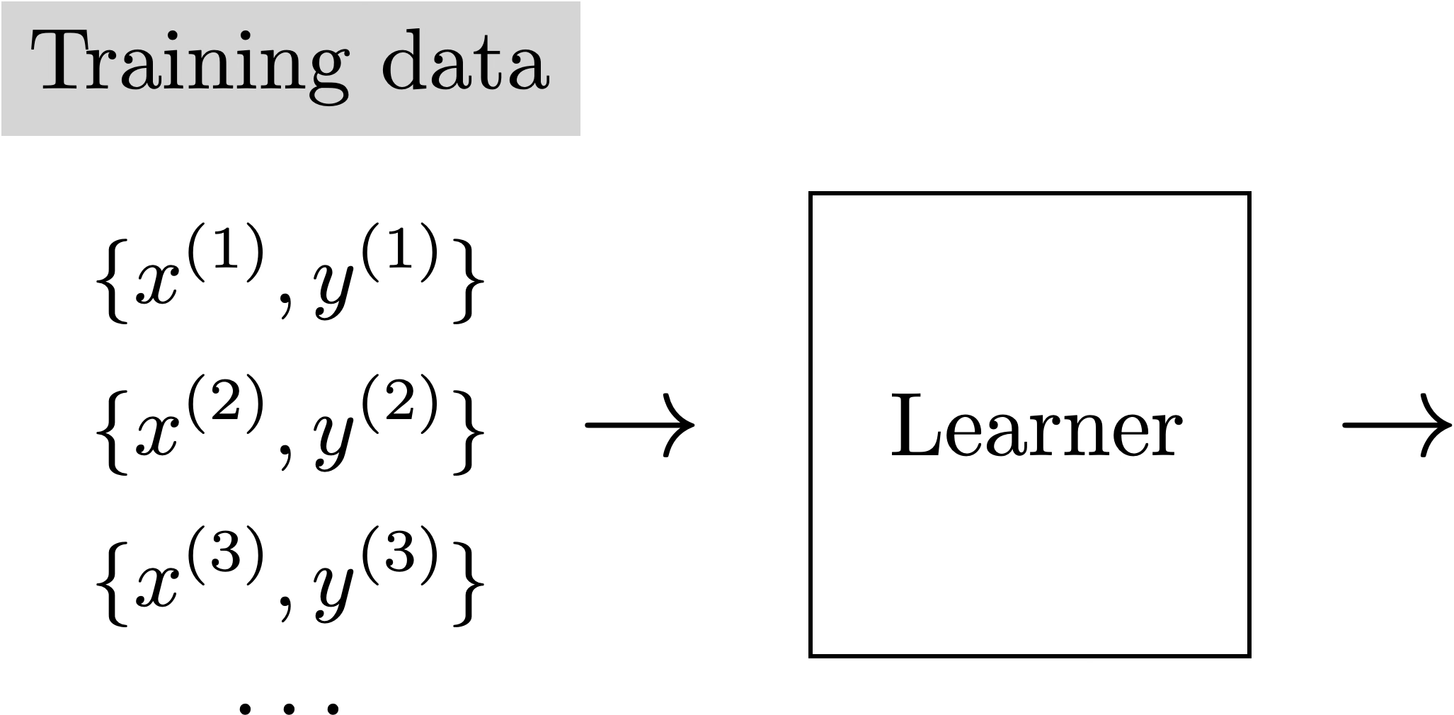
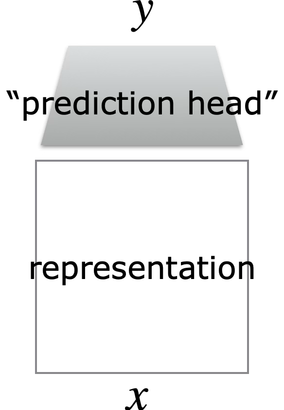
\(f: X \rightarrow Y\)
Supervised Learning
"Good"
Representation
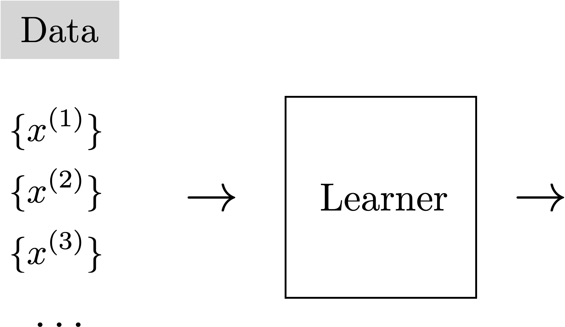
Unsupervised Learning
Training Data
🧠
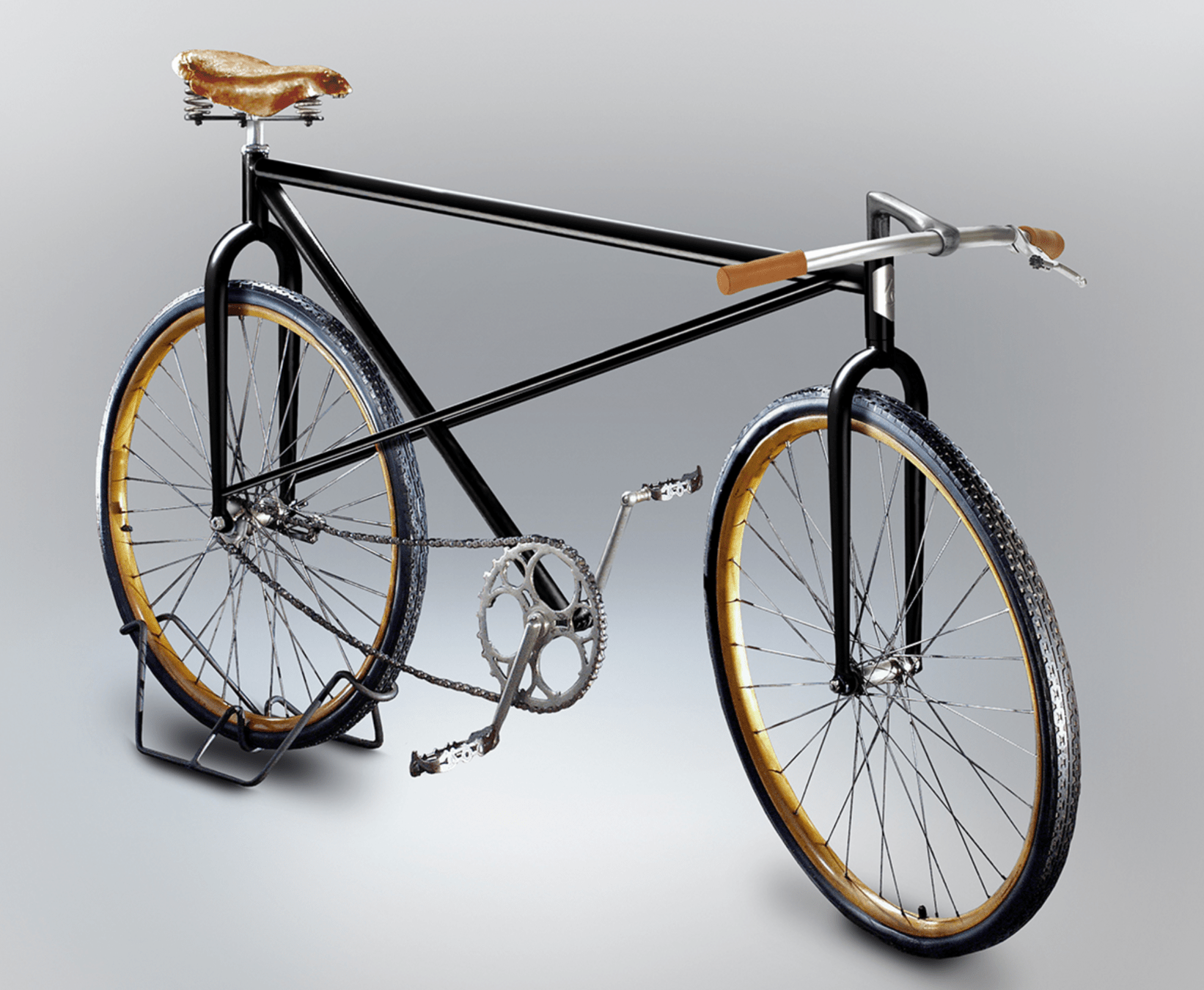
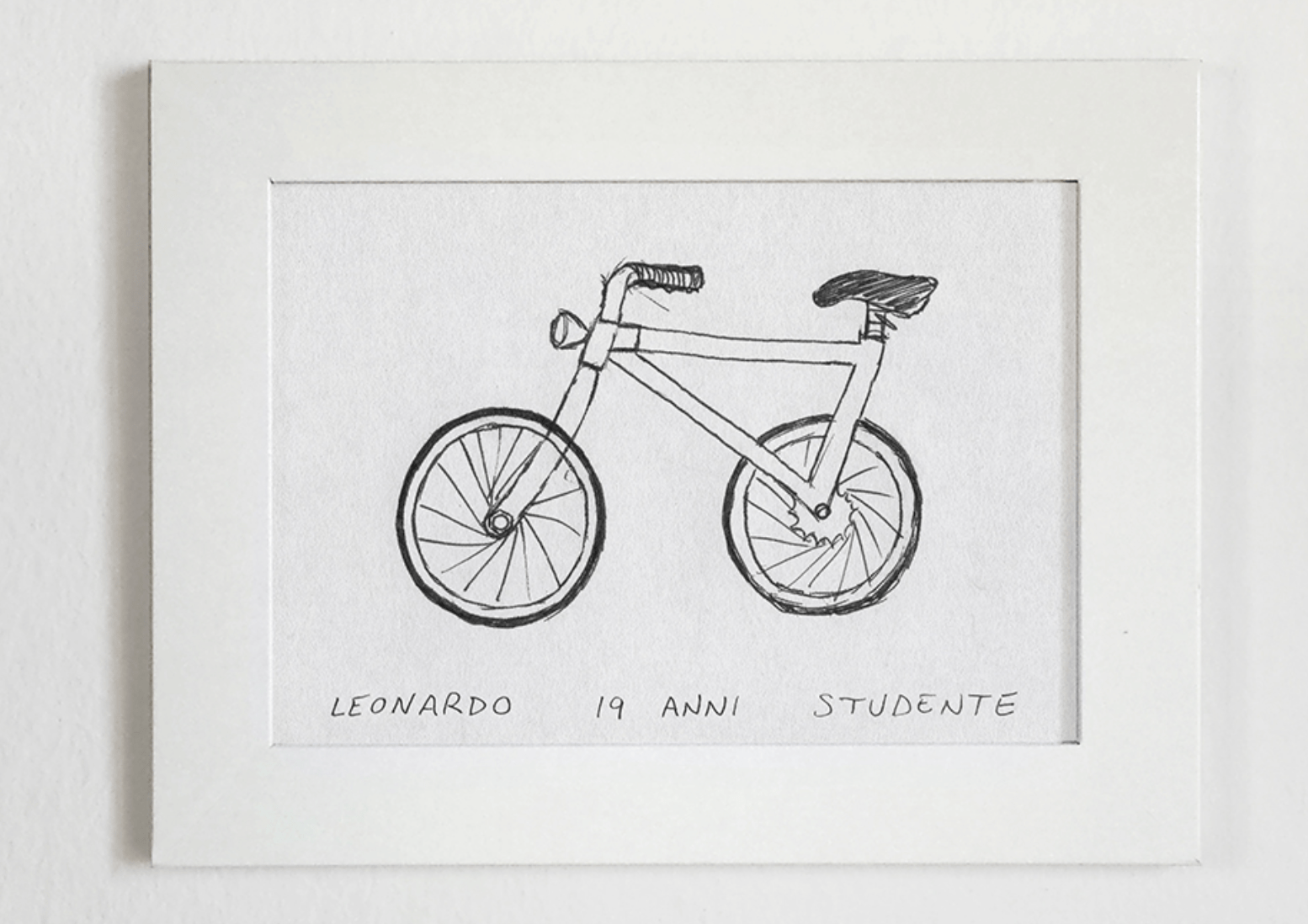
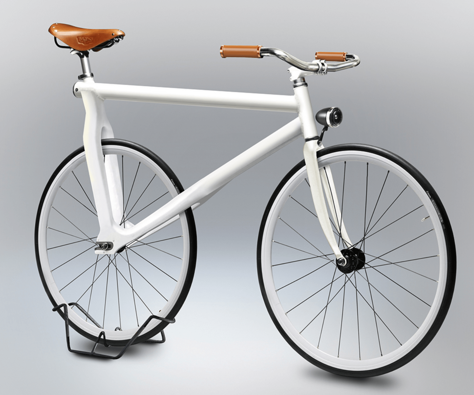
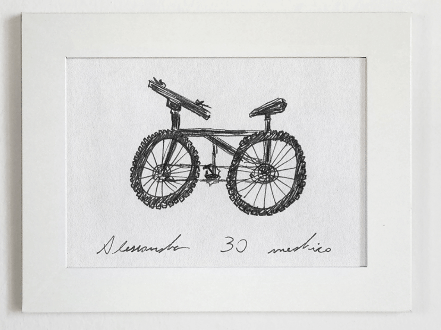
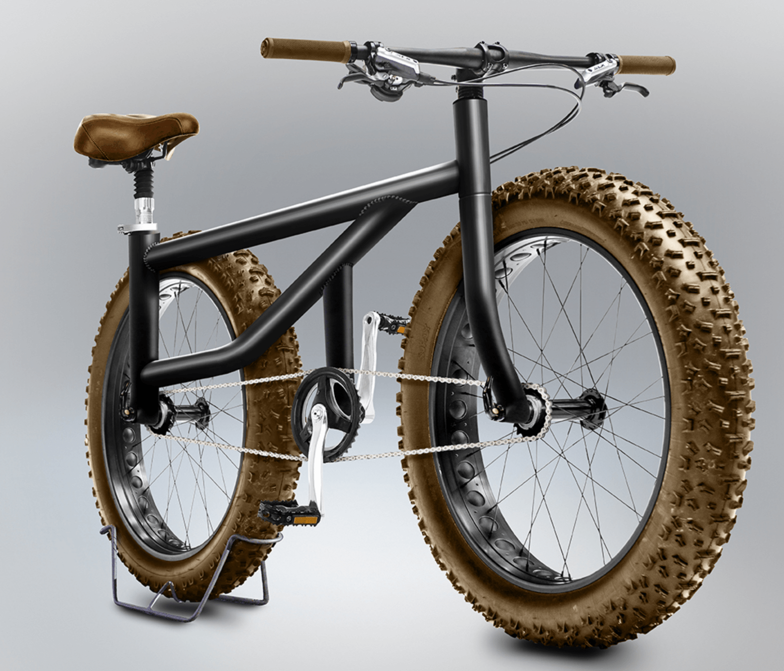
humans also learn representations
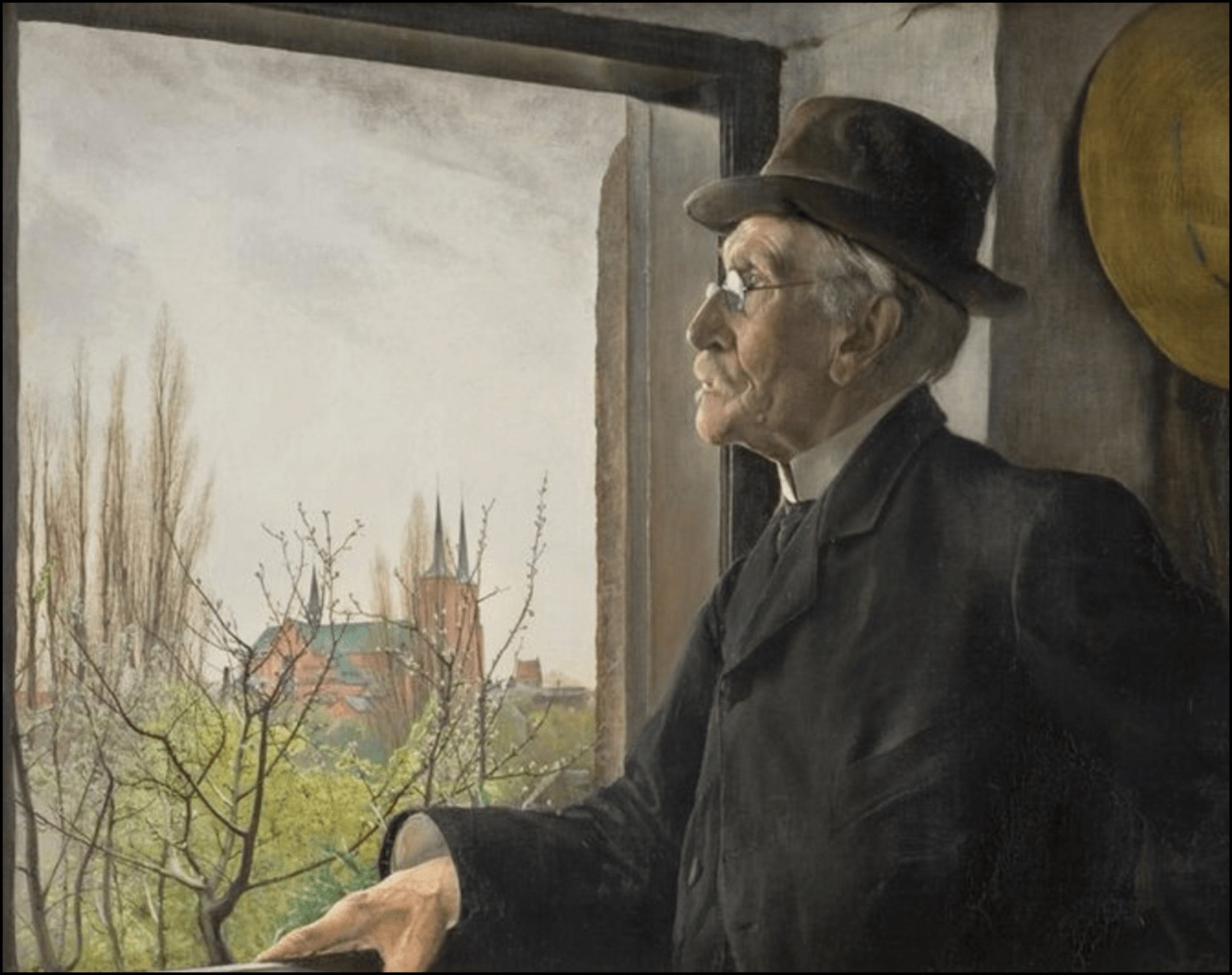
"I stand at the window and see a house, trees, sky. Theoretically I might say there were 327 brightnesses and nuances of colour. Do I have "327"? No. I have sky, house, and trees.”
— Max Wertheimer, 1923
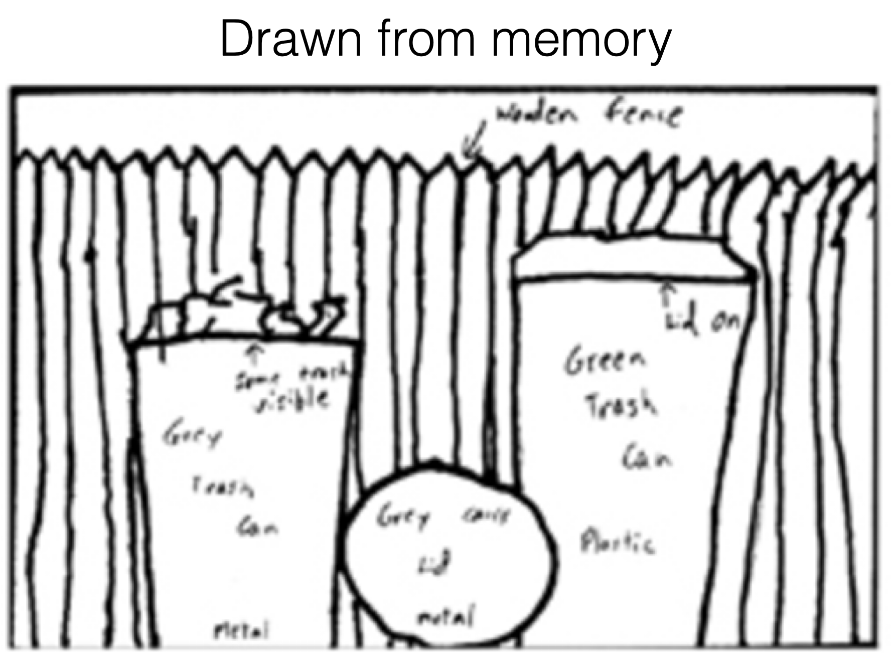
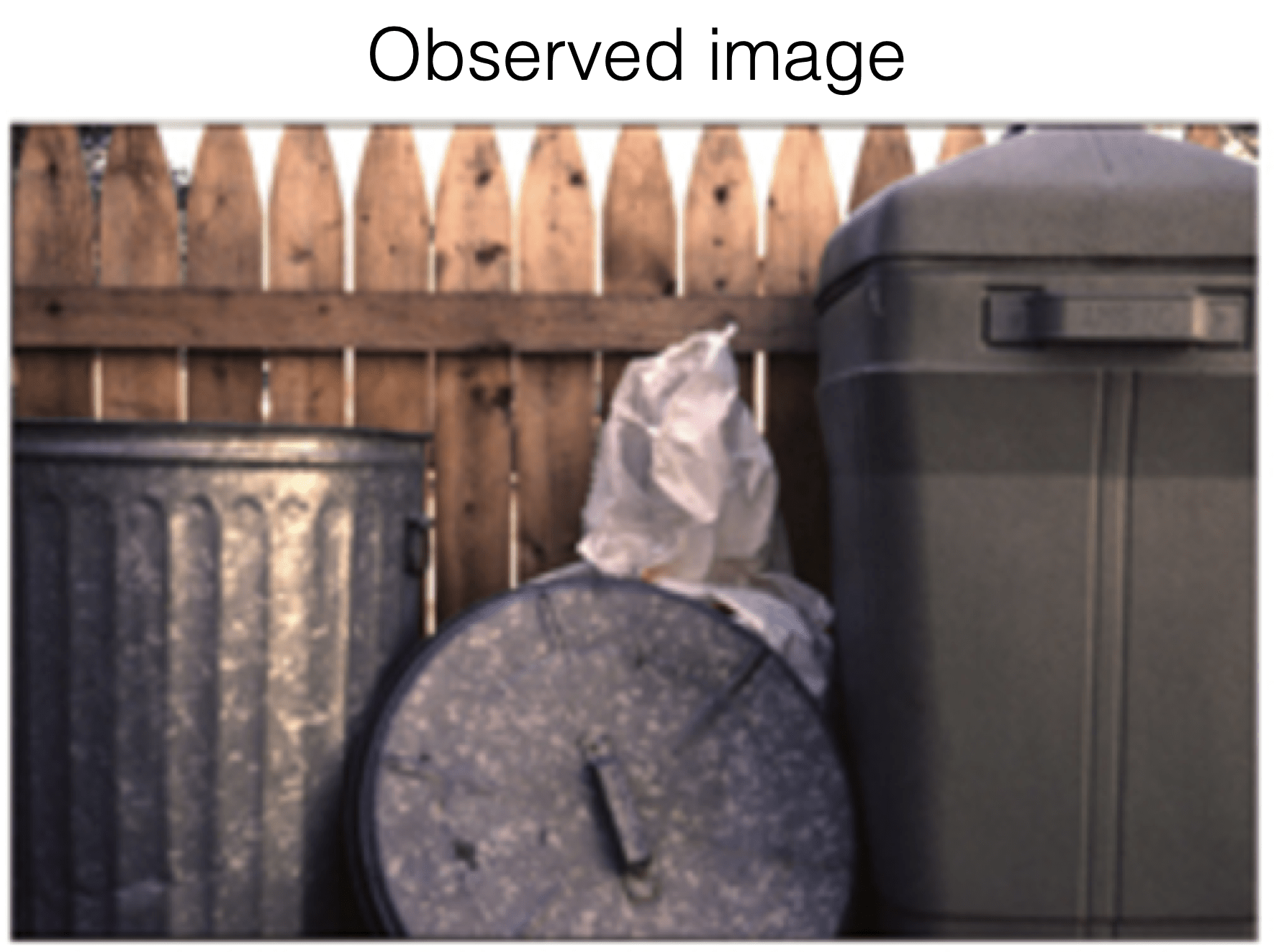
Good representations are:
- Compact (minimal)
- Explanatory (roughly sufficient)
[See “Representation Learning”, Bengio 2013, for more commentary]
[Bartlett, 1932]
[Intraub & Richardson, 1989]
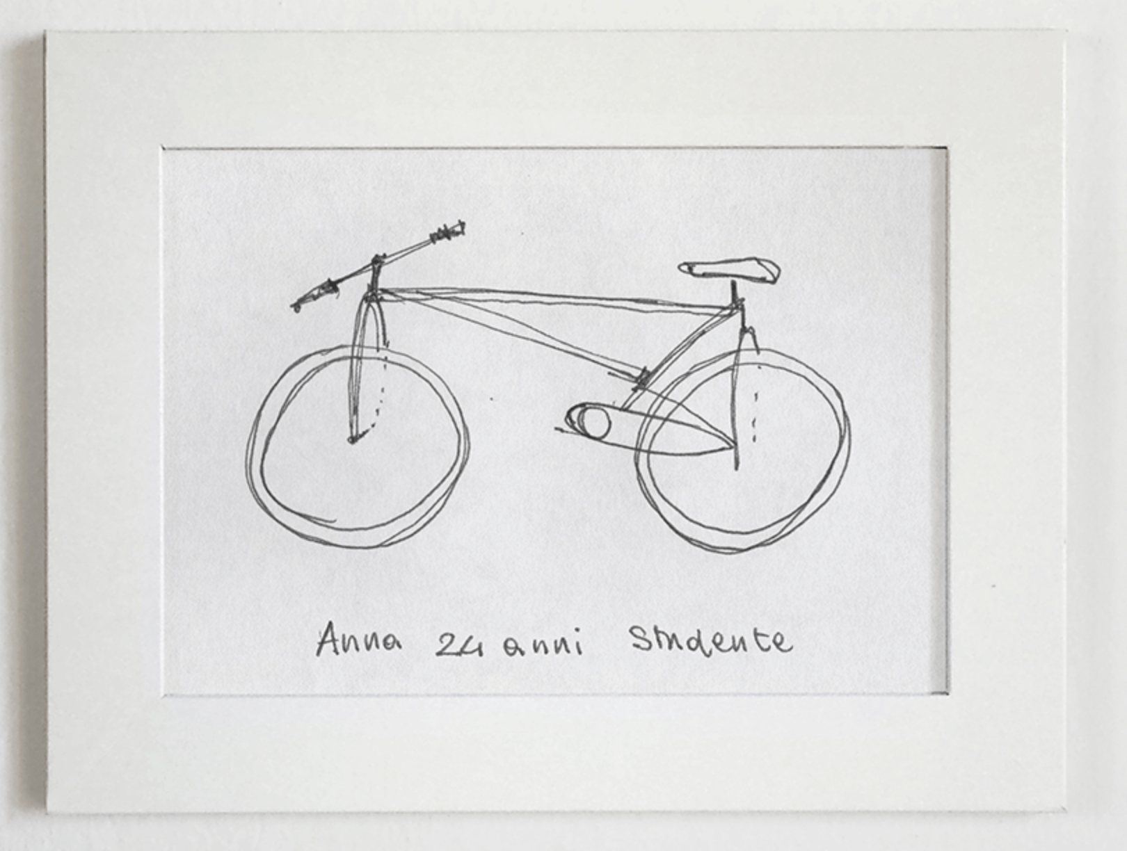
[https://www.behance.net/gallery/35437979/Velocipedia]
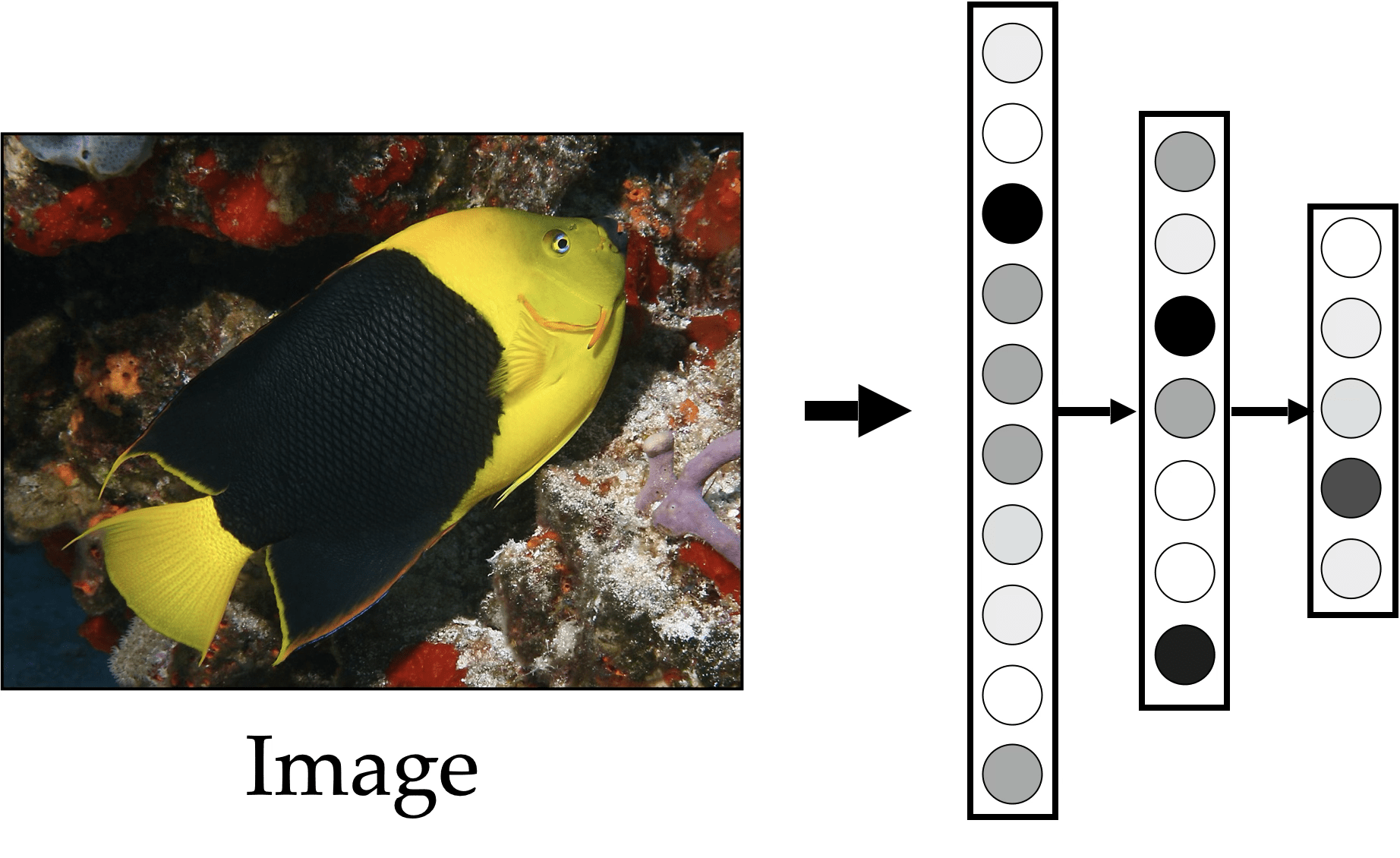
compact representation/embedding
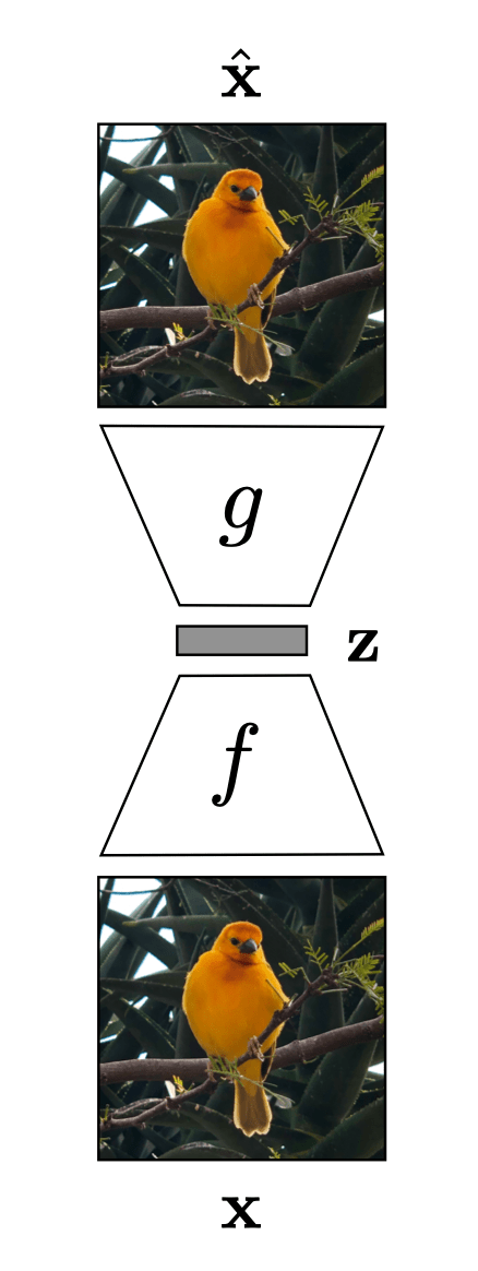
Auto-encoder
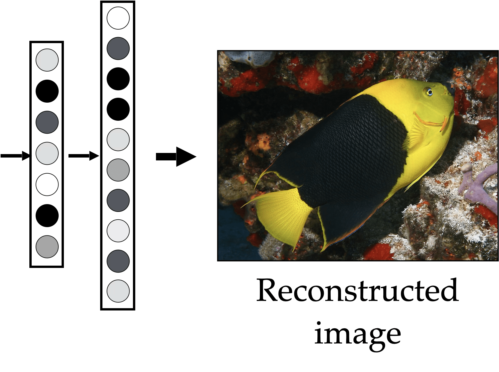
Auto-encoder
"What I cannot create, I do not understand." Feynman
Auto-encoder
\underbrace{\hspace{1cm}}
\underbrace{\hspace{1cm}}
encoder
decoder
bottleneck
Auto-encoder
x
\tilde{x}=\text{NN}(x;W)
\min_{W} ||x - \tilde{x}||^2
Auto-encoder
Training Data
\left\{{x}^{(i)}\right\}_{i=1}^n
loss/objective
\mathcal{L}(F(\mathbf{x}), \mathbf{x})=\|F(\mathbf{x})-\mathbf{x}\|^2
hypothesis class
A model
\(f\)
F=g \circ h: \mathbb{R}^d \rightarrow \mathbb{R}^m \rightarrow \mathbb{R}^d
h
g
\(m<d\)
- Compact (minimal)
- Explanatory (roughly sufficient)
- Disentangled (independent factors)
- Interpretable
- Make subsequent problem solving easy
[See “Representation Learning”, Bengio 2013, for more commentary]
Auto-encoders try to achieve these
\left\{
\begin{array}{l}
\\
\\
\end{array}
\right.
\left\{
\begin{array}{l}
\\
\\
\\
\end{array}
\right.
these may just emerge as well
Good representations are:
https://www.tensorflow.org/text/tutorials/word2vec
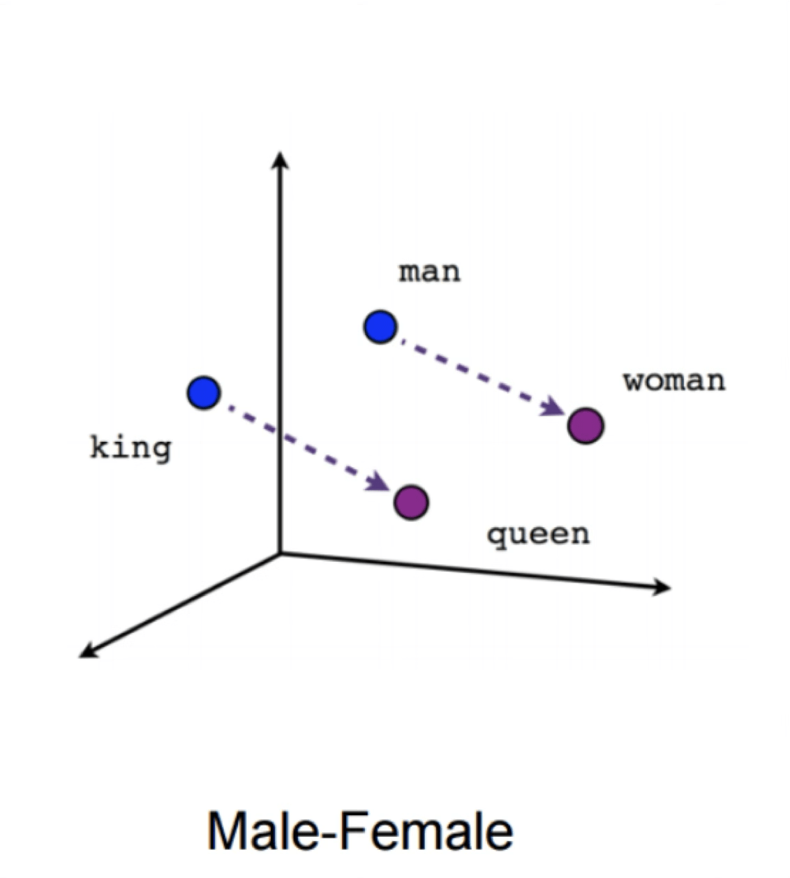
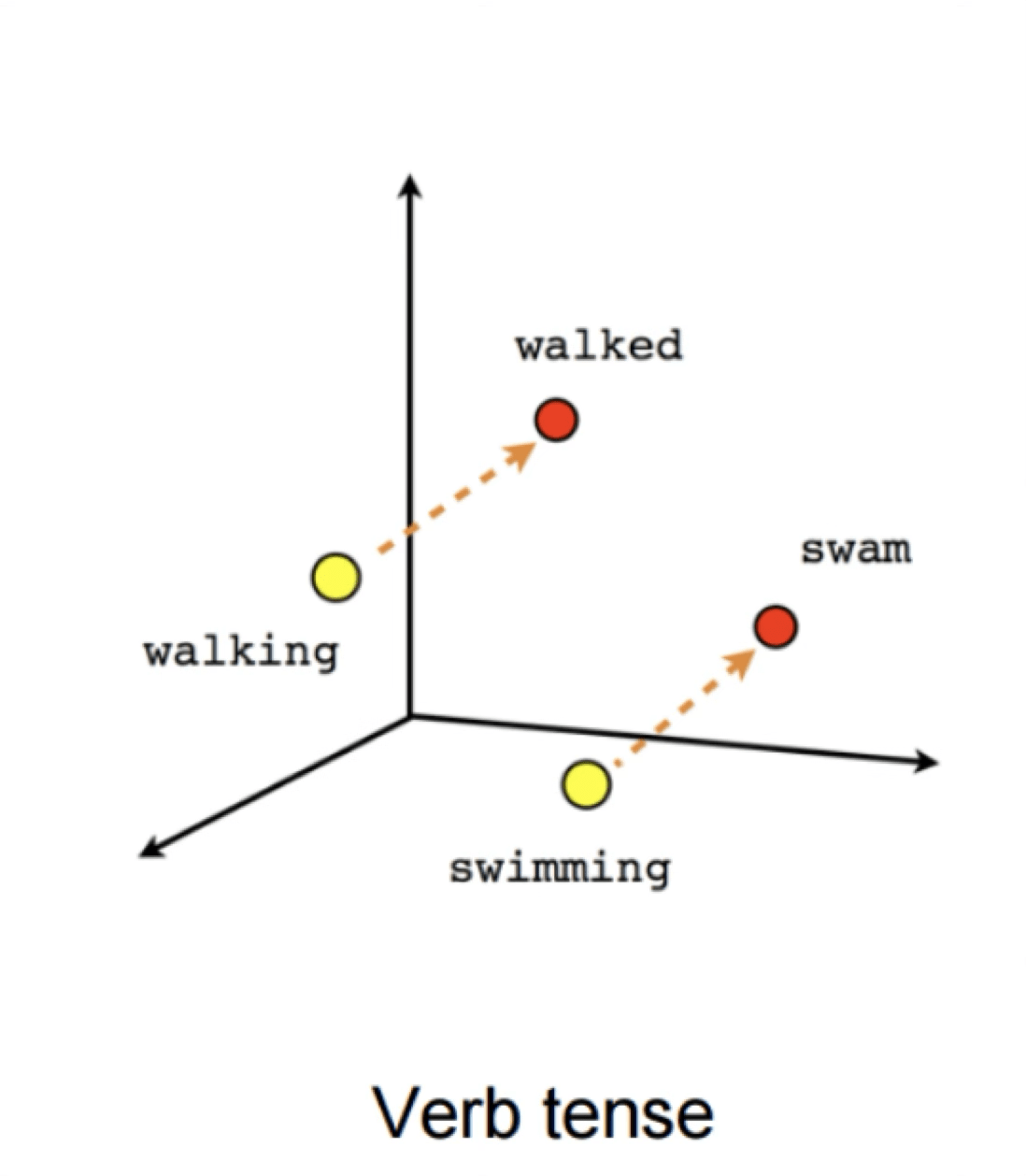
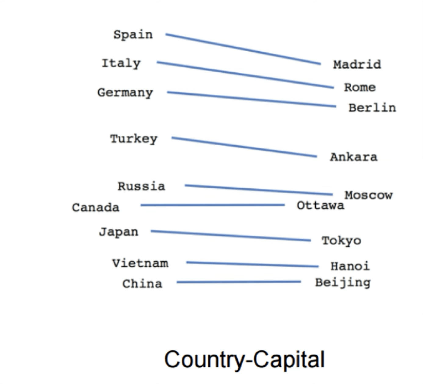
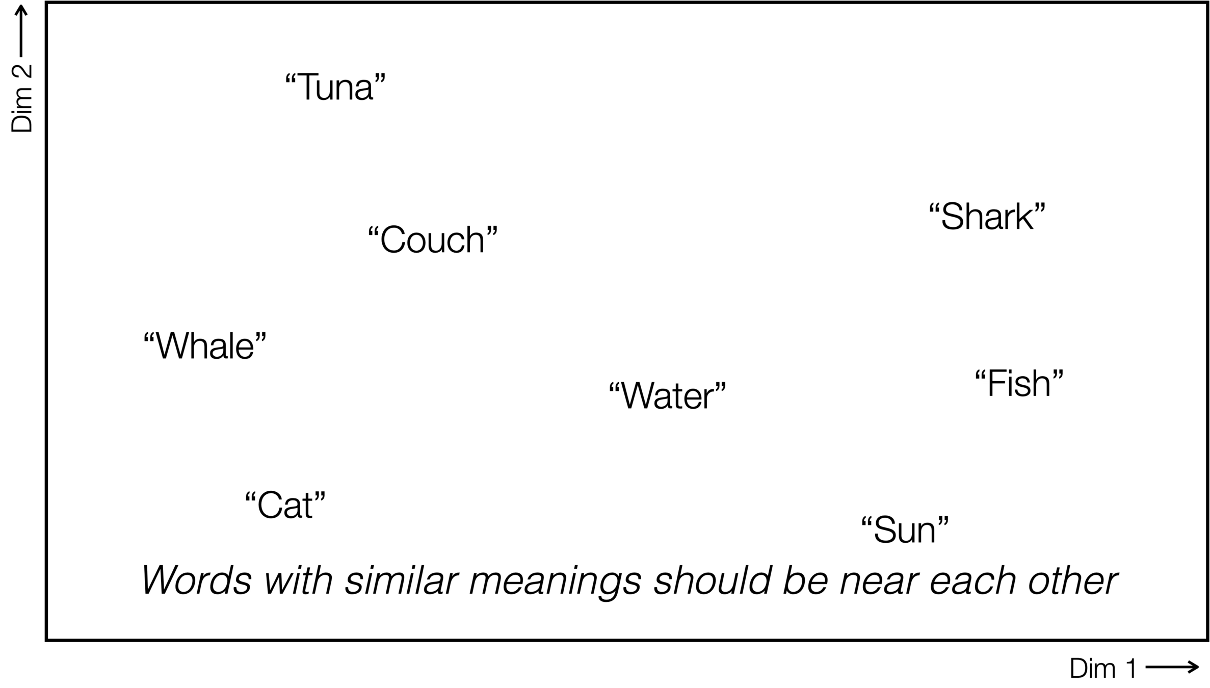
Word2Vec
verb tense
gender
X = Vector(“Paris”) – vector(“France”) + vector(“Italy”) \(\approx\) vector("Rome")
“Meaning is use” — Wittgenstein
[Mikolov et al., 2013]
Can help downstream tasks:
- sentiment analysis
- machine translation
- info retrieval
Word2Vec
[video edited from 3b1b]
embedding
a
robot
must
obey
\left\{
\begin{array}{l}
\\
\\
\\
\end{array}
\right.
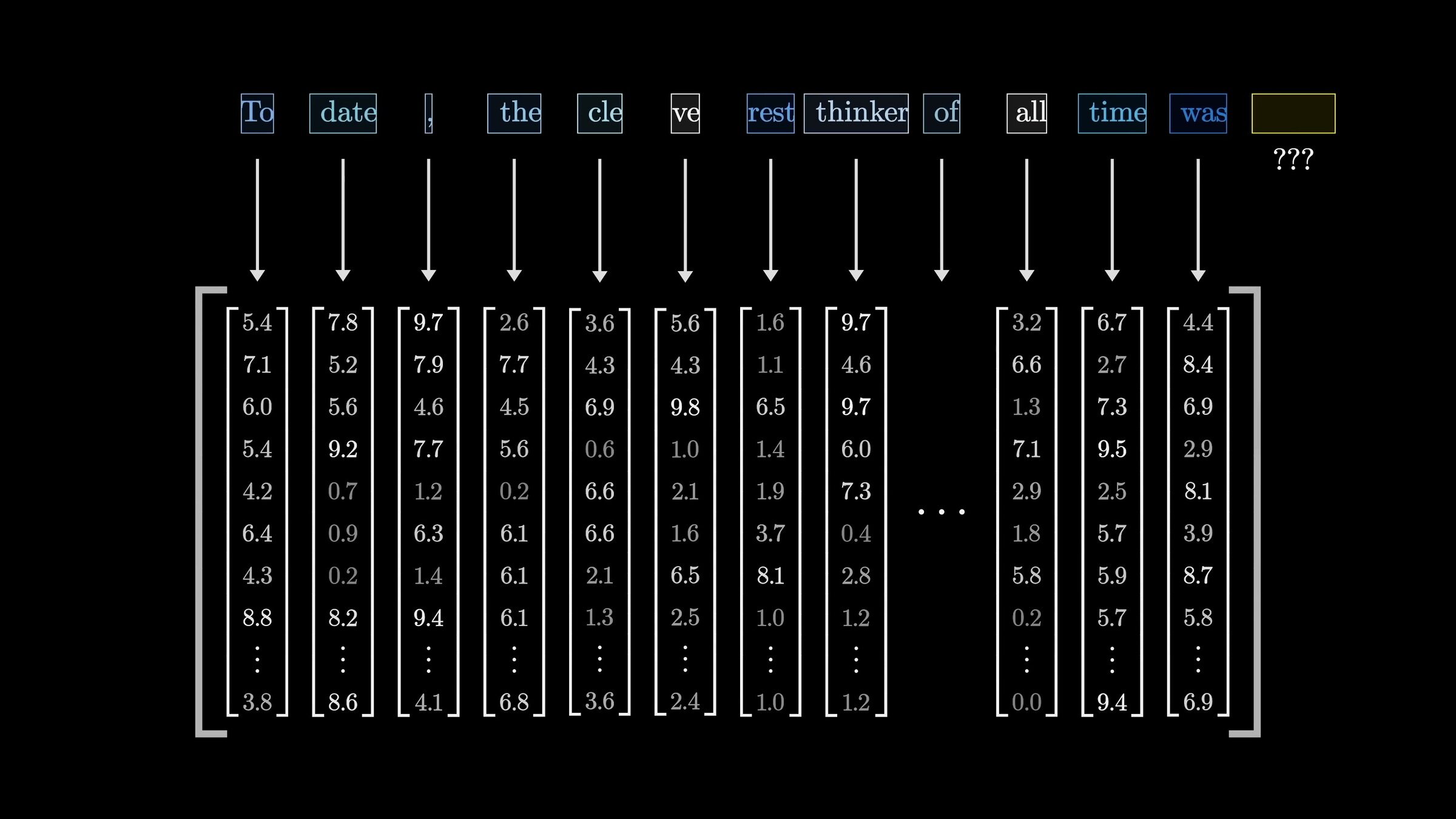
distribution over the vocabulary
Transformer
"A robot must obey the orders given it by human beings ..."
push for Prob("robot") to be high
push for Prob("must") to be high
push for Prob("obey") to be high
push for Prob("the") to be high
\(\dots\)
\(\dots\)
\(\dots\)
\(\dots\)
a
robot
must
obey
input embedding
output embedding
\(\dots\)
\(\dots\)
\(\dots\)
\(\dots\)
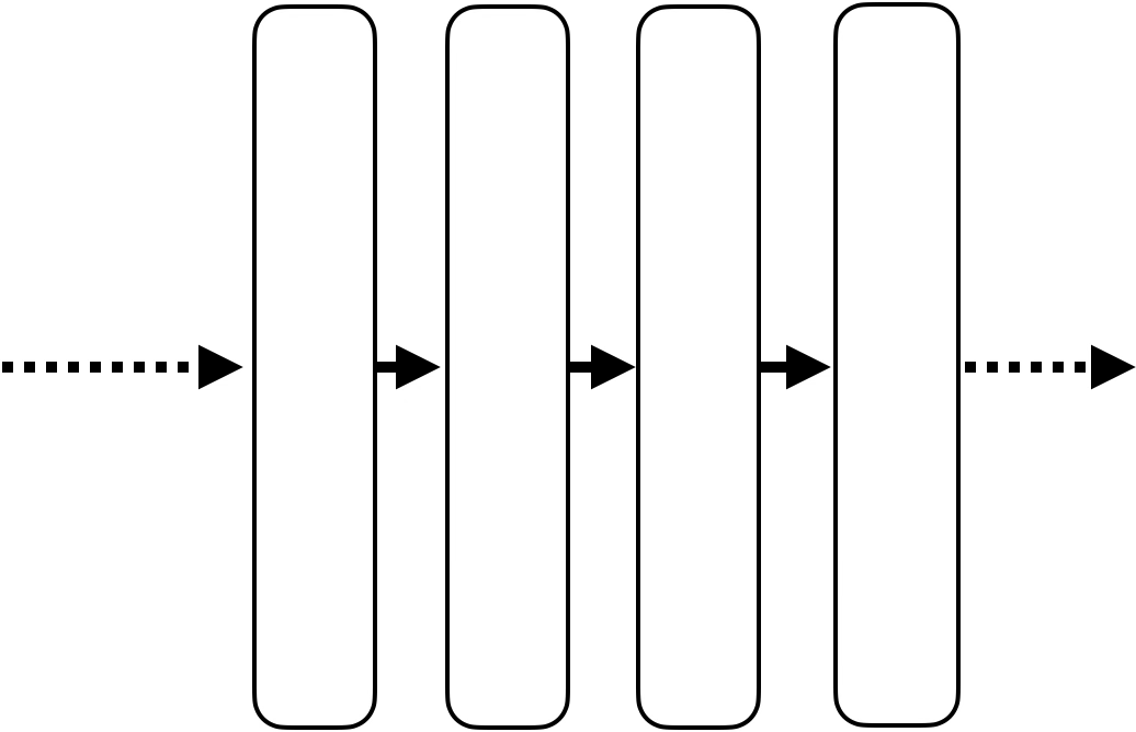
transformer block
transformer block
transformer block
\left\{
\begin{array}{l}
\\
\\
\\
\\
\end{array}
\right.
\(L\) blocks
\(\dots\)
a
robot
must
obey
input embedding
output embedding
\(\dots\)
\(\dots\)
\(\dots\)
\(\dots\)
\(\dots\)
transformer block
transformer block
transformer block
x^{(1)}
x^{(2)}
x^{(3)}
x^{(4)}
A sequence of \(n\) tokens, each token in \(\mathbb{R}^{d}\)
a
robot
must
obey
input embedding
\(\dots\)
transformer block
transformer block
transformer block
x^{(1)}
x^{(2)}
x^{(3)}
x^{(4)}
output embedding
\(\dots\)
\(\dots\)
\(\dots\)
\(\dots\)
a
robot
must
obey
input embedding
output embedding
transformer block
\(\dots\)
\(\dots\)
\(\dots\)
attention layer
fully-connected network
x^{(1)}
x^{(2)}
x^{(3)}
x^{(4)}
\(\dots\)
[video edited from 3b1b]
[video edited from 3b1b]
a
robot
must
obey
input embedding
output embedding
transformer block
\(\dots\)
\(\dots\)
\(\dots\)
\(\dots\)
attention layer
fully-connected network
x^{(1)}
x^{(2)}
x^{(3)}
W_k
W_v
W_q
the usual weights
x^{(4)}
attention mechanism
[image edited from 3b1b]
\(n\)
\underbrace{\hspace{5.98cm}}
\left\{
\begin{array}{l}
\\
\\
\\
\\
\\
\\
\\
\end{array}
\right.
\(d\)
input embedding (e.g. via a fixed encoder)
[video edited from 3b1b]
[video edited from 3b1b]
[image edited from 3b1b]
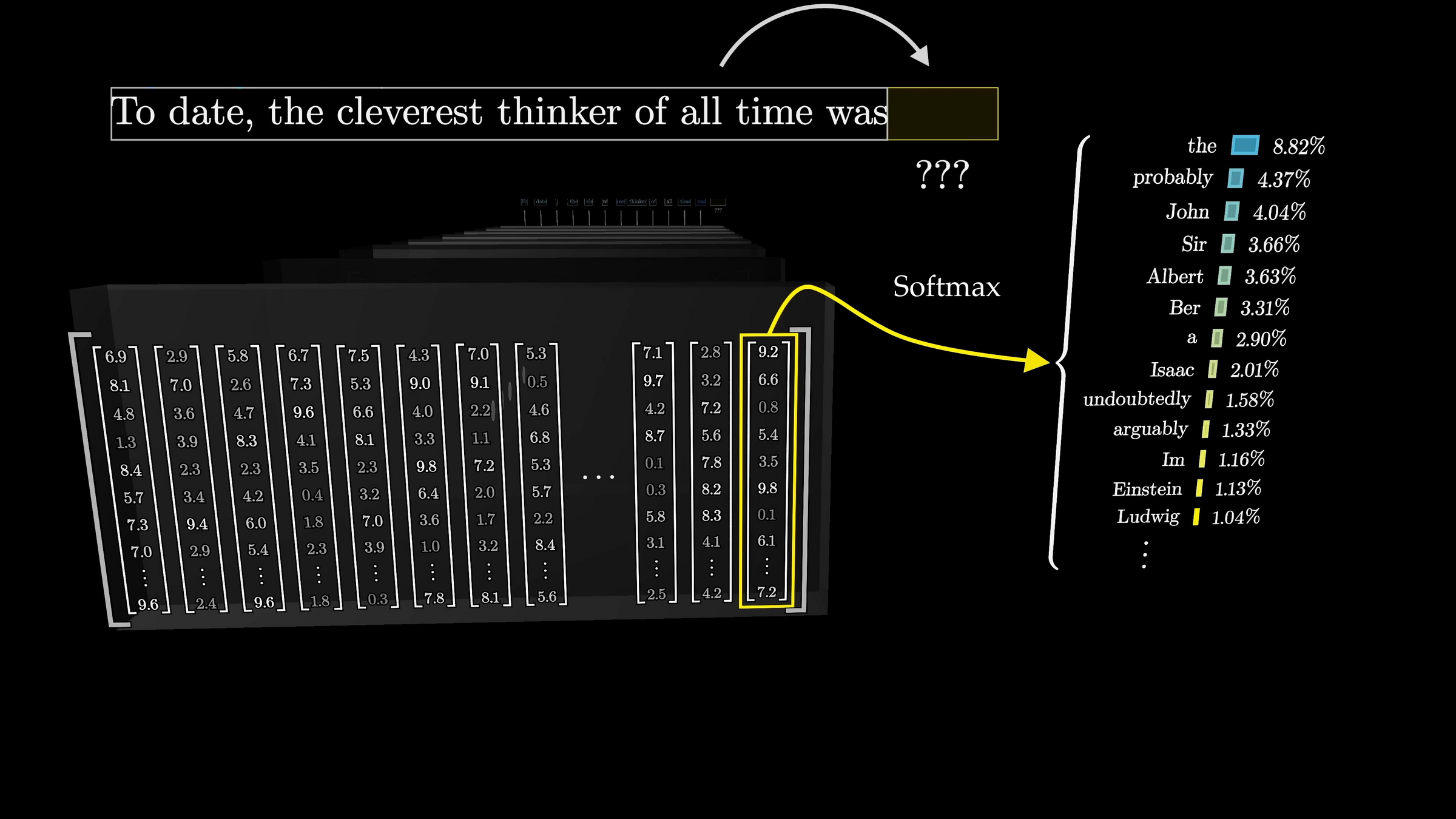
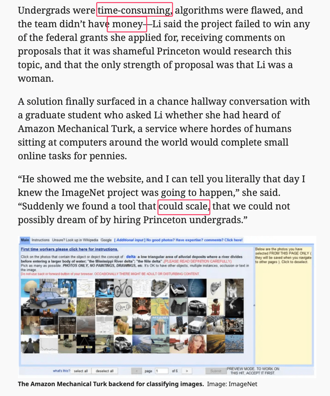
Cross-entropy loss encourages the internal weights update so as to make this probability higher
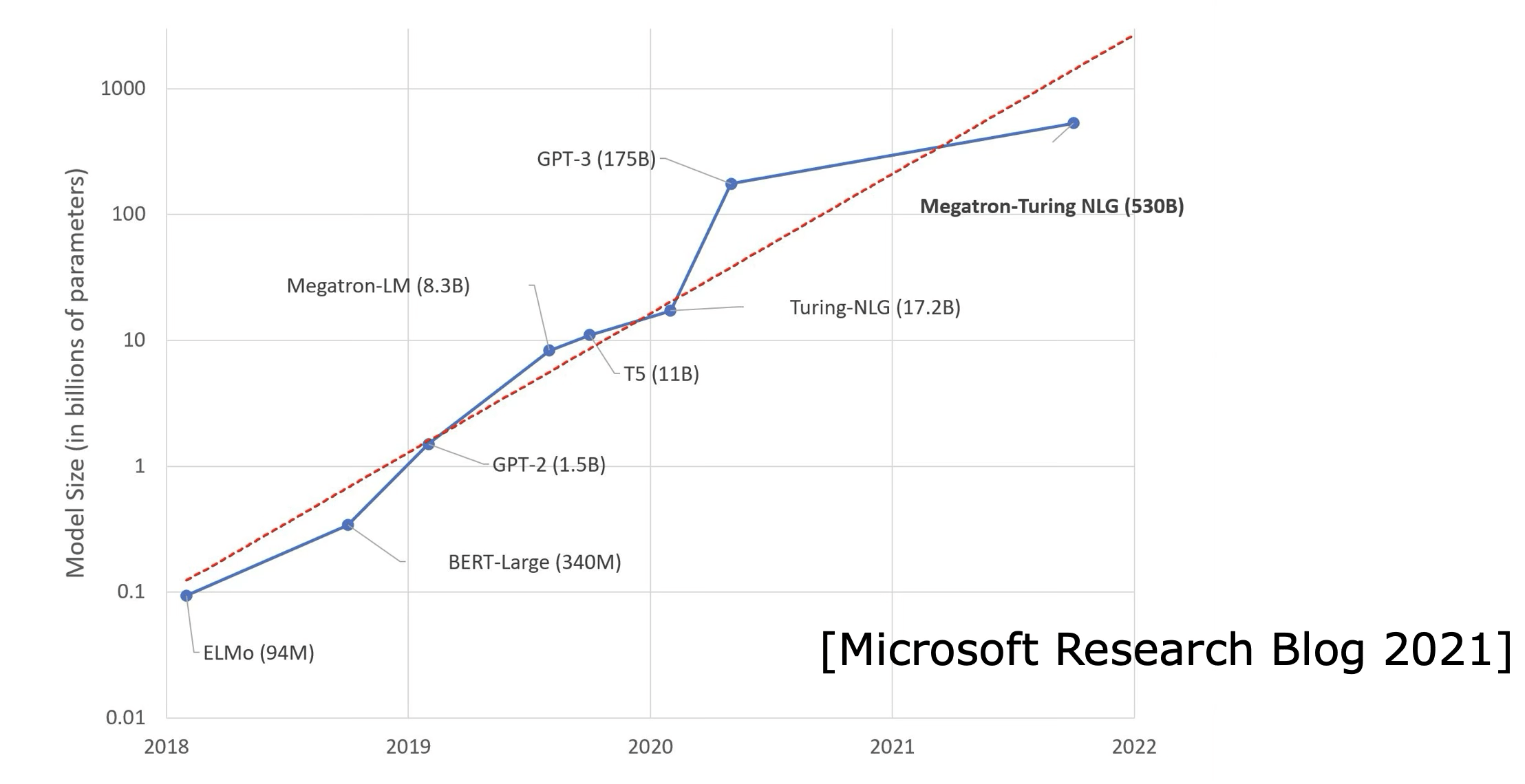
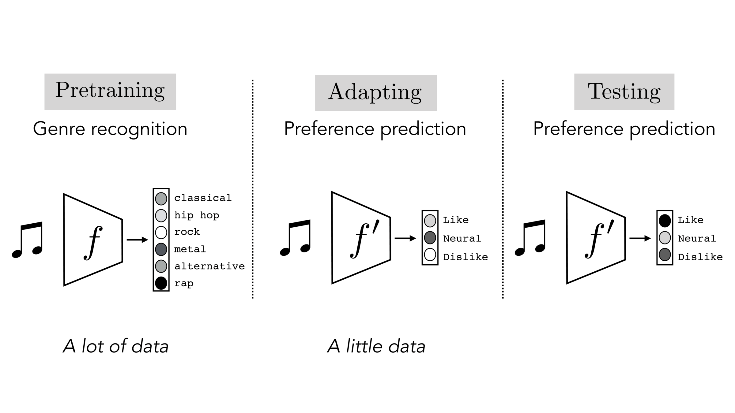
Foundation Models
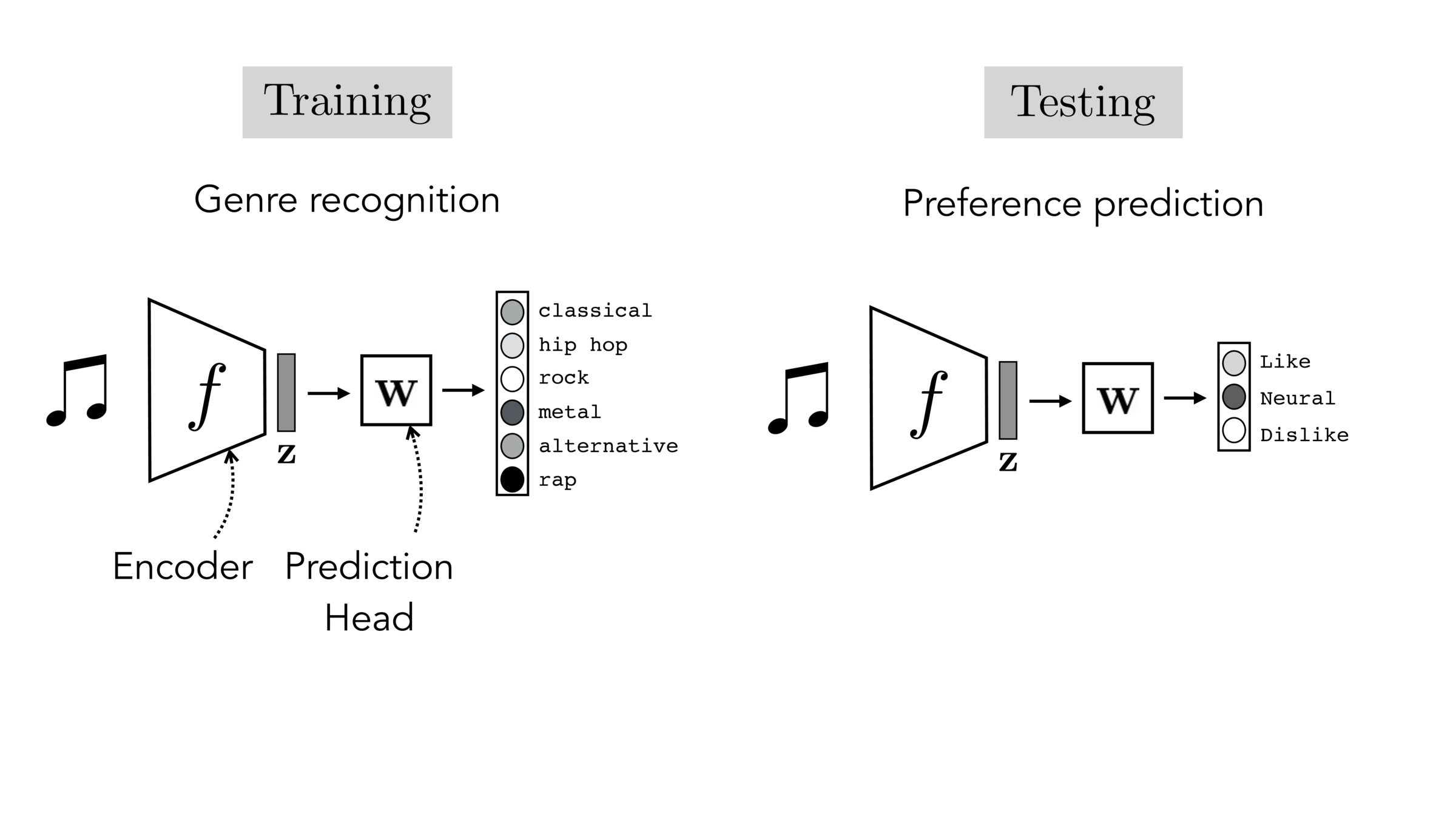
Often, what we will be “tested” on is not what we were trained on.
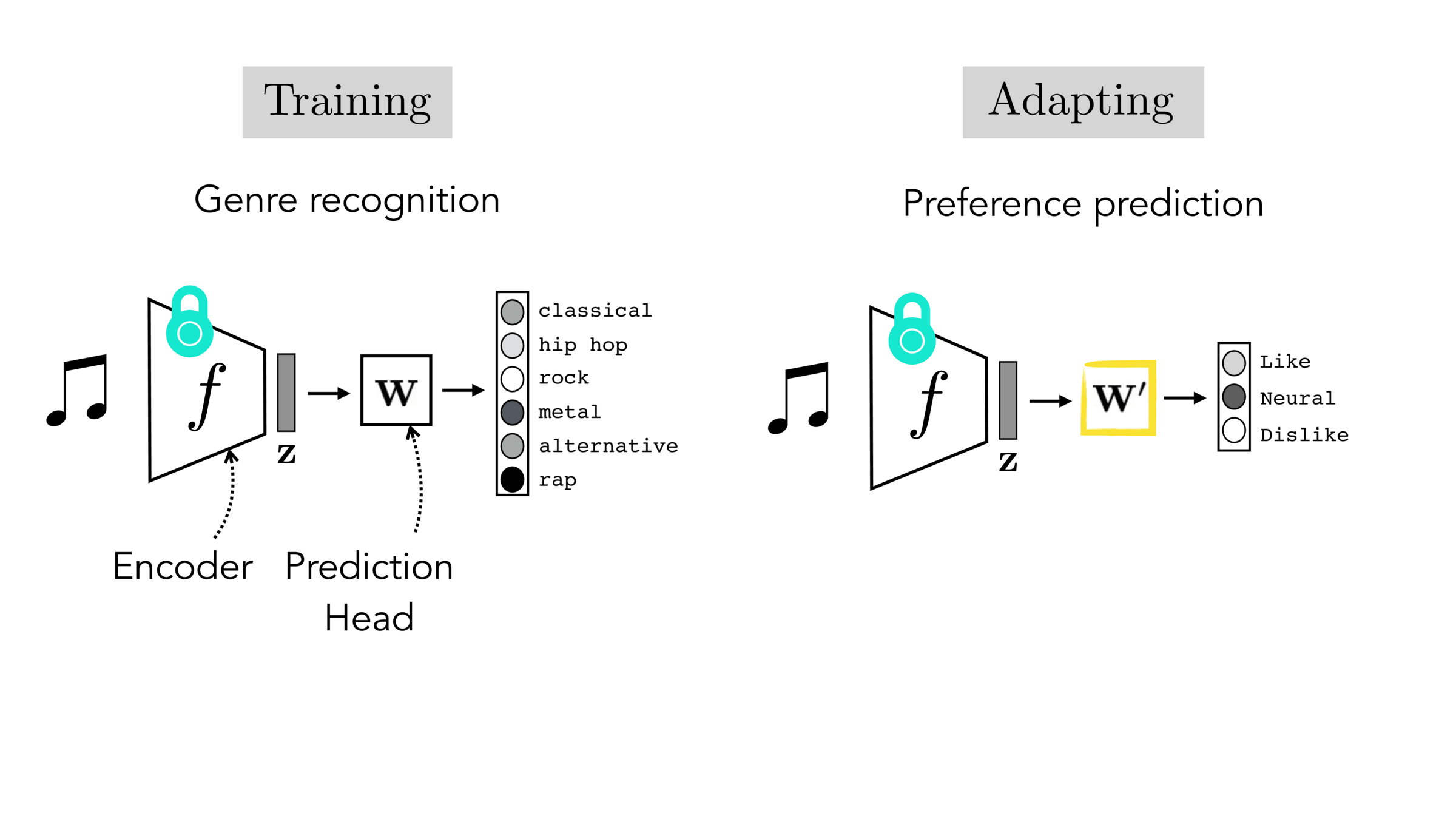
Final-layer adaptation: freeze \(f\), train a new final layer to new target data
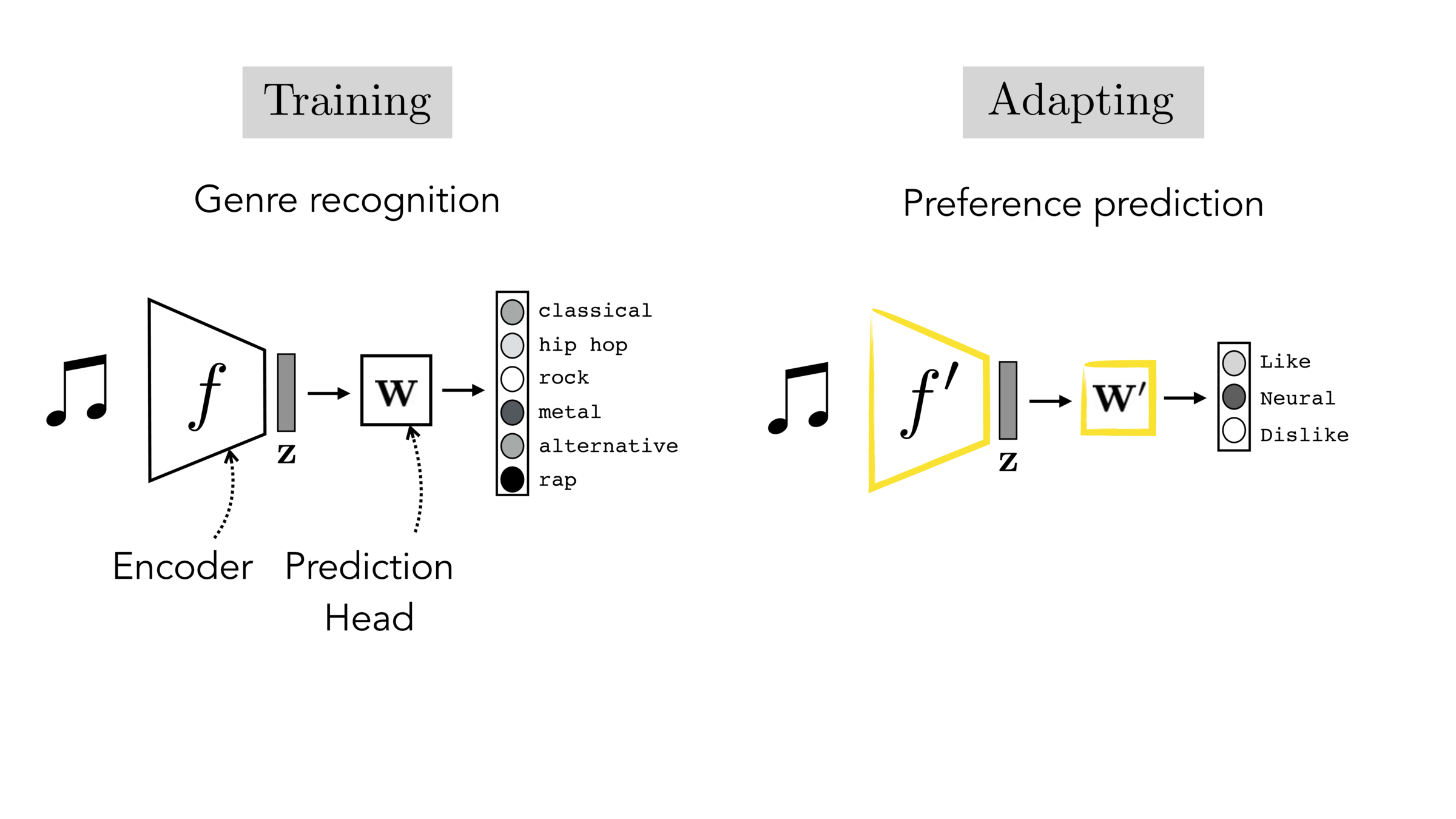
Finetuning: initialize \(f’\) as \(f\), then continue training for \(f'\) as well, on new target data
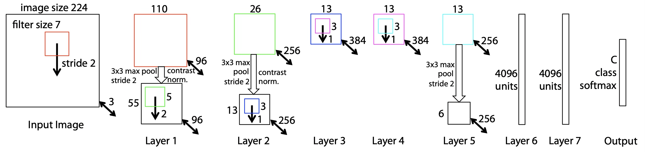
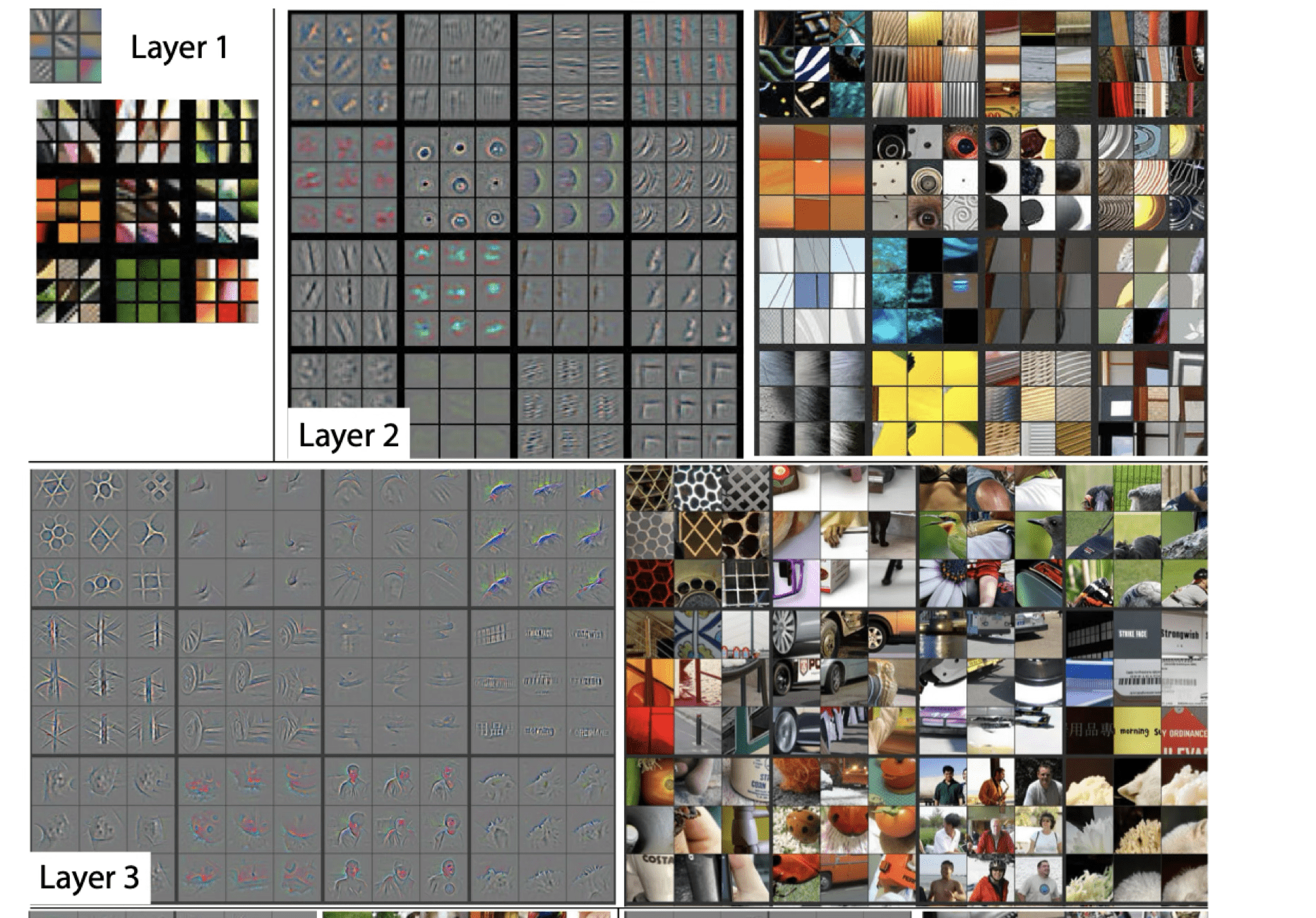
[Zeiler et al. 2013]
E.g., features from a model pre-trained on image net can be reused for medical images
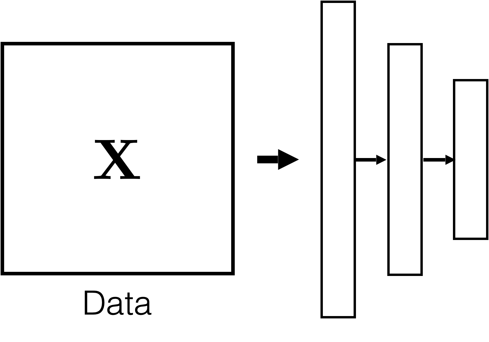
Label prediction (supervised learning)
Features
Label
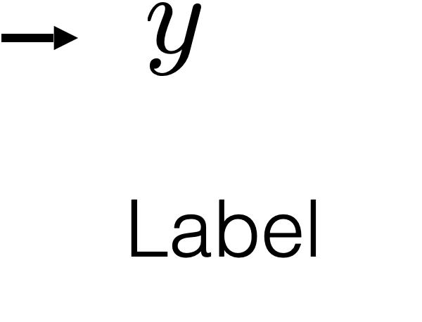
Feature reconstruction (unsupervised learning)
Features
Reconstructed Features
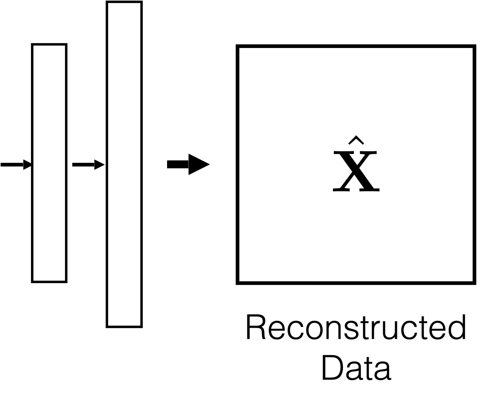
Partial
features
Other partial
features
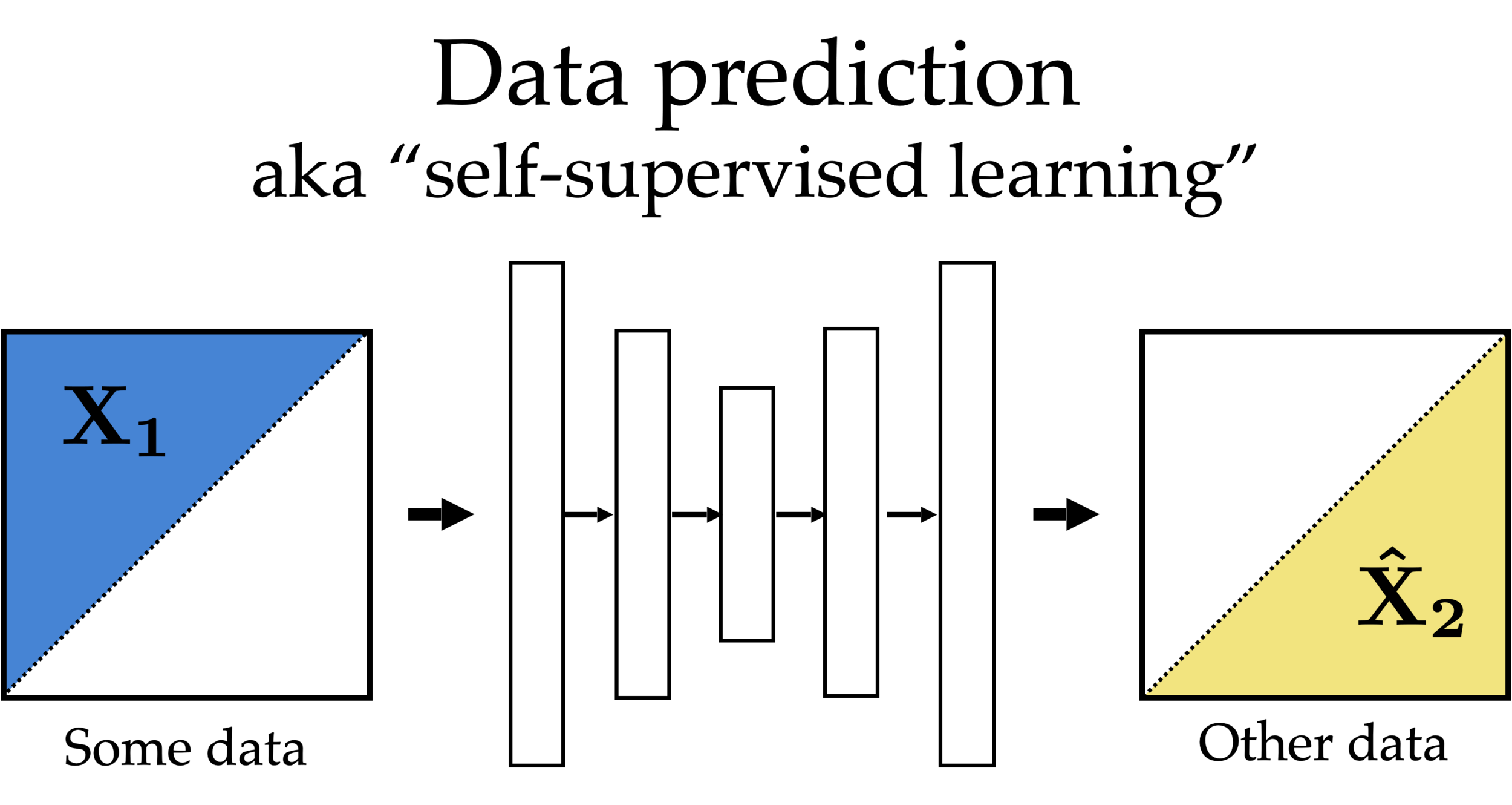
Feature reconstruction (self-supervised learning)
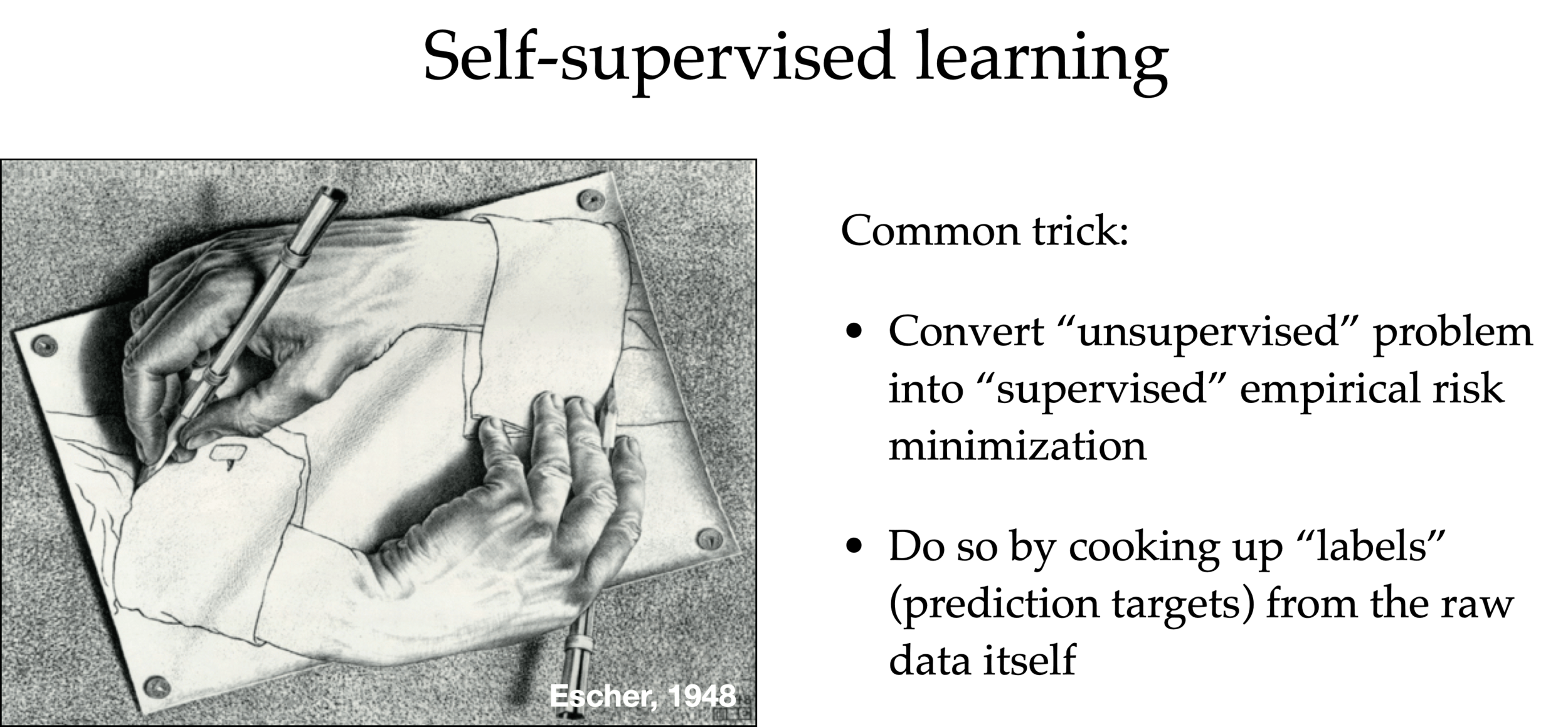
Self-supervised learning
Common trick:
- Convert “unsupervised” problem into “supervised” setup
- Do so by cooking up “labels” (prediction targets) from the raw data itself — called pretext task
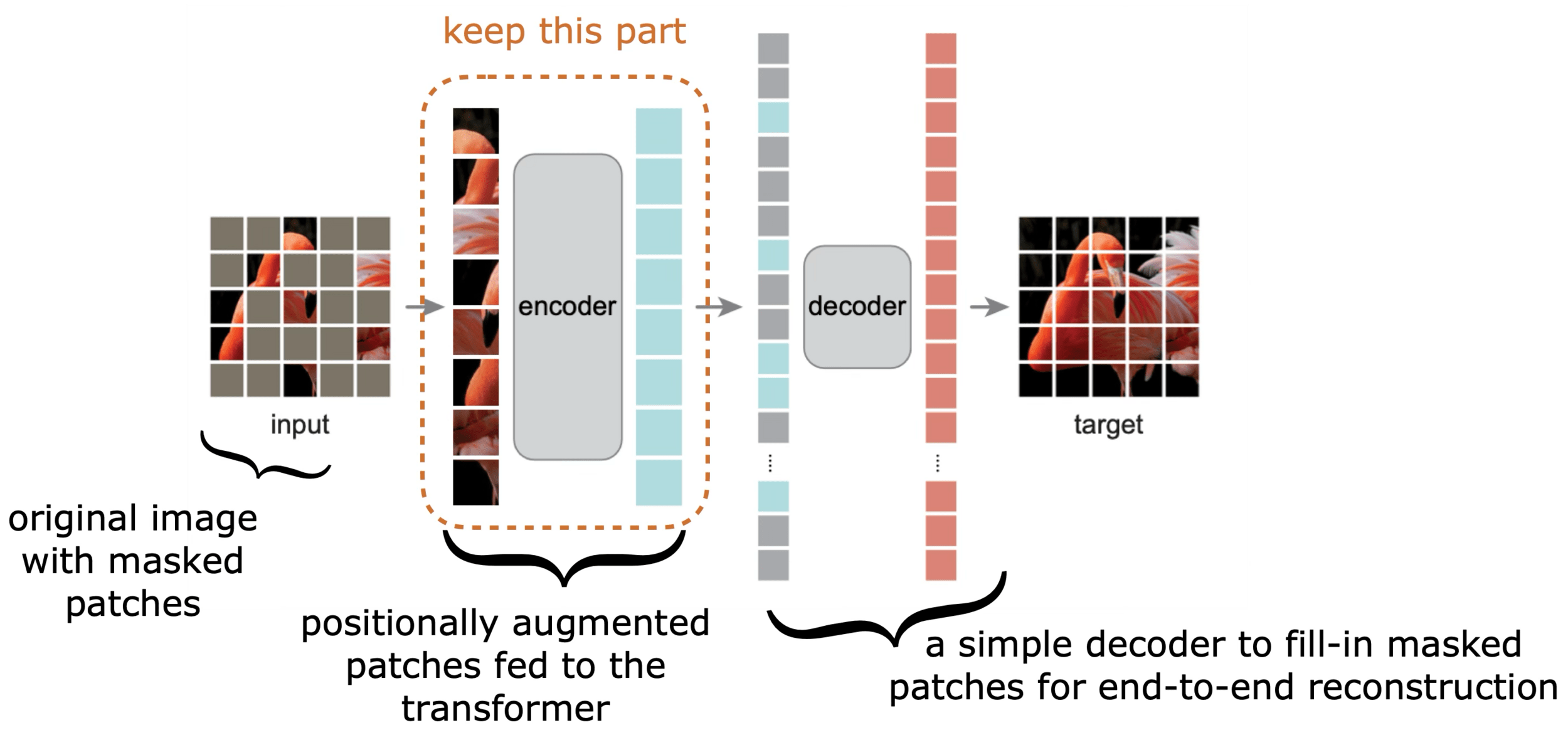
Masked Auto-encoder
[He, Chen, Xie, et al. 2021]
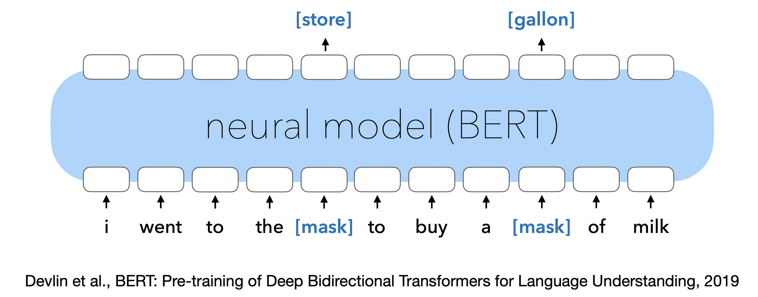
Masked Auto-encoder
[Devlin, Chang, Lee, et al. 2019]
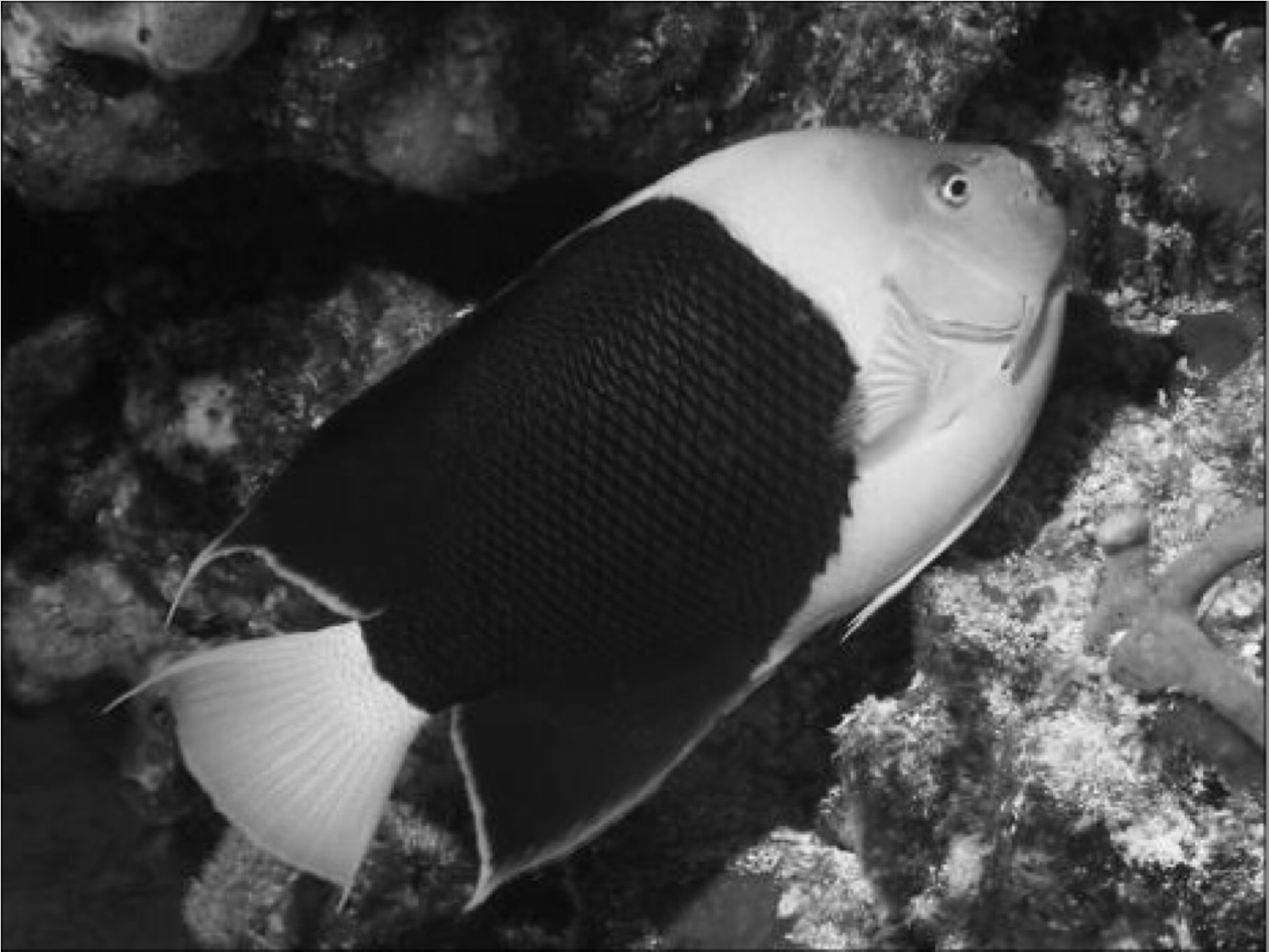
[Zhang, Isola, Efros, ECCV 2016]

predict color from gray-scale
[Zhang, Isola, Efros, ECCV 2016]
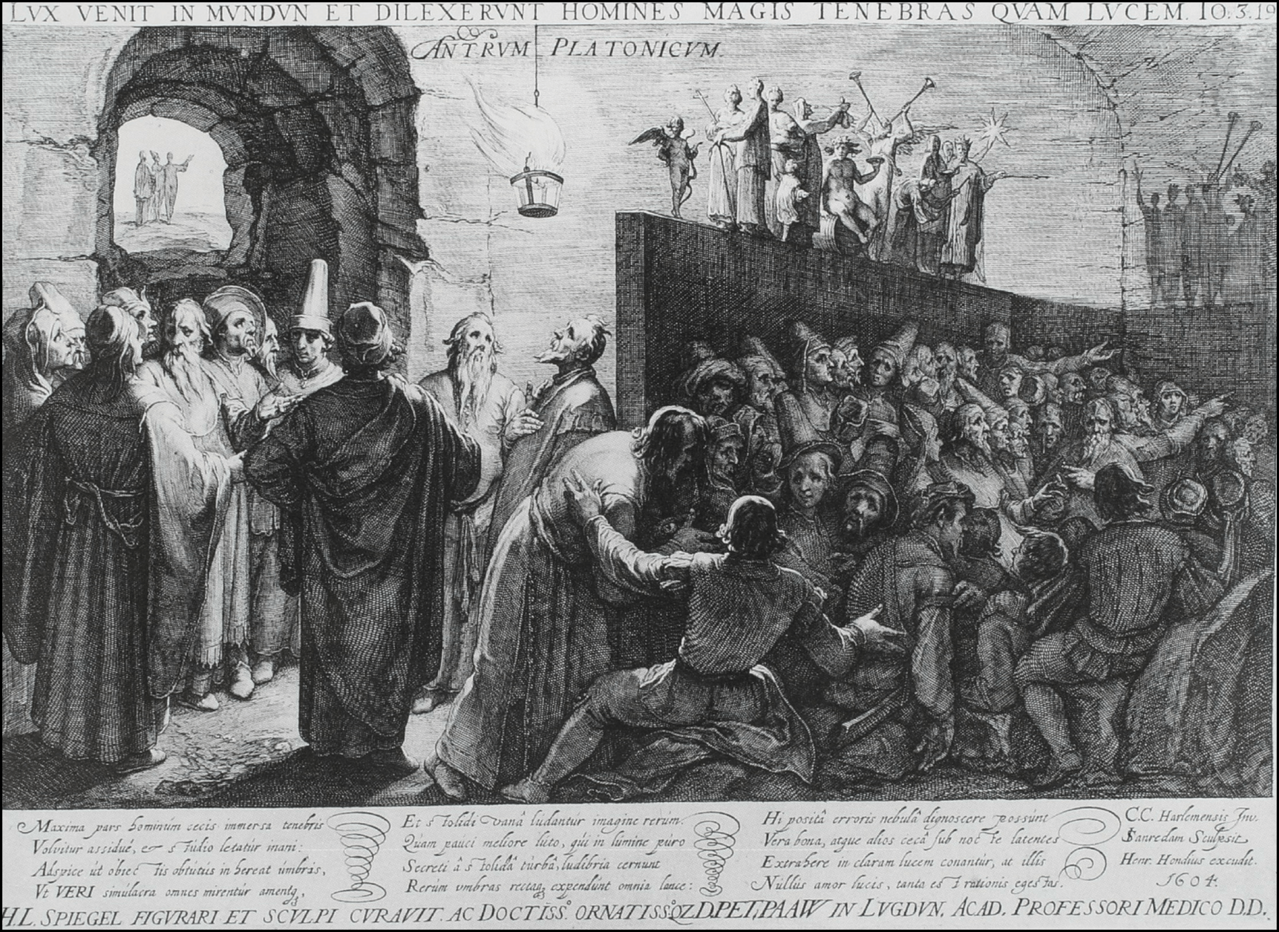


The allegory of the cave

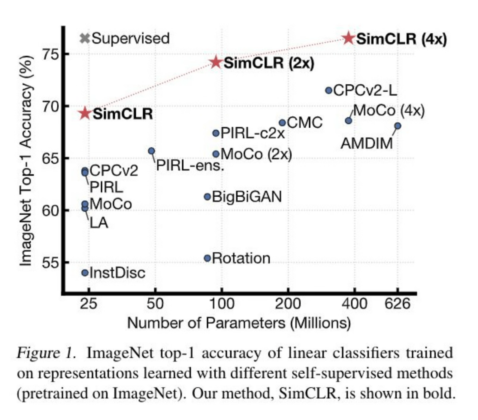
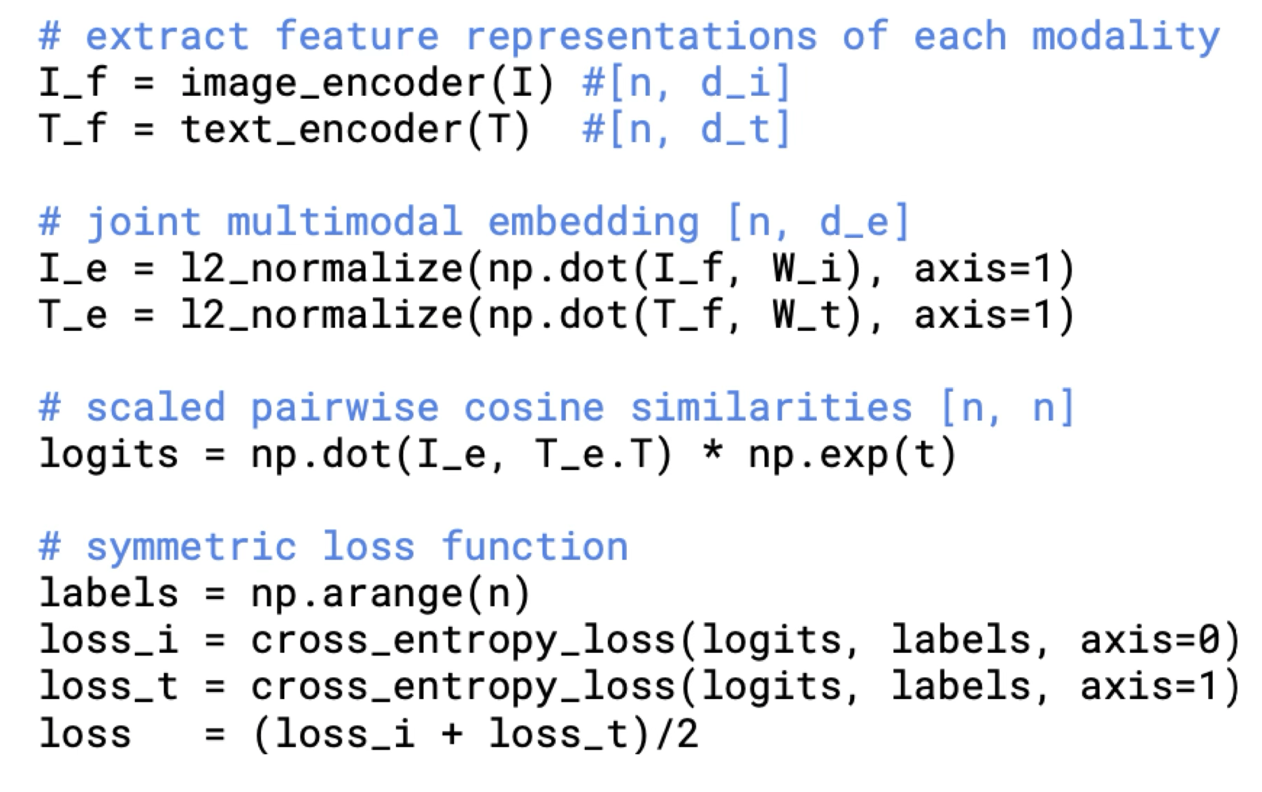
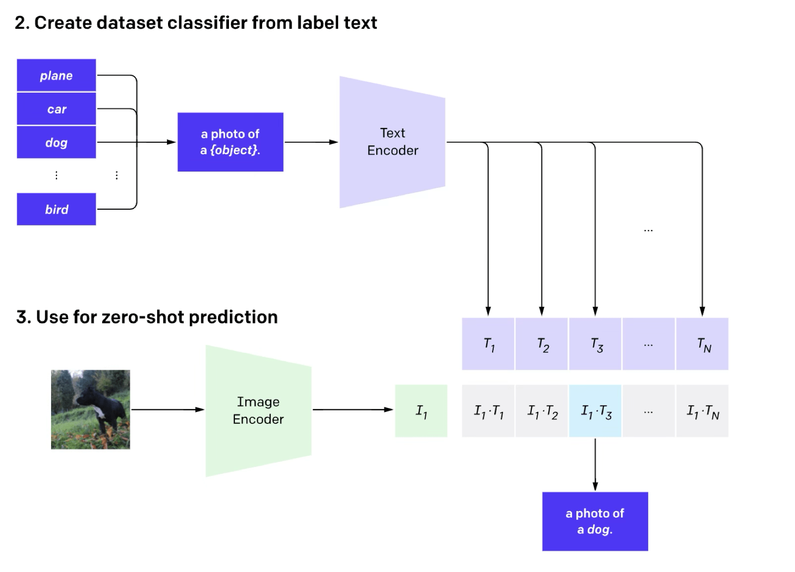
Contrastive learning
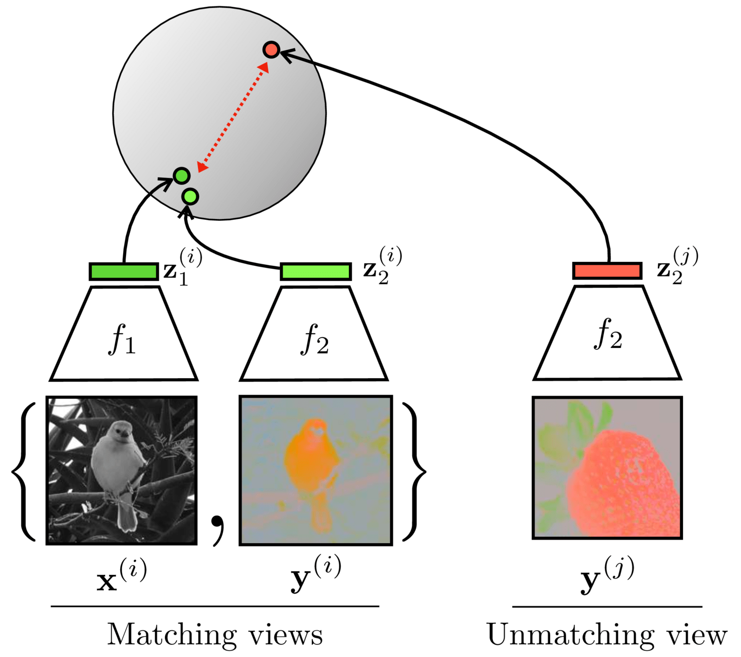
Contrastive learning
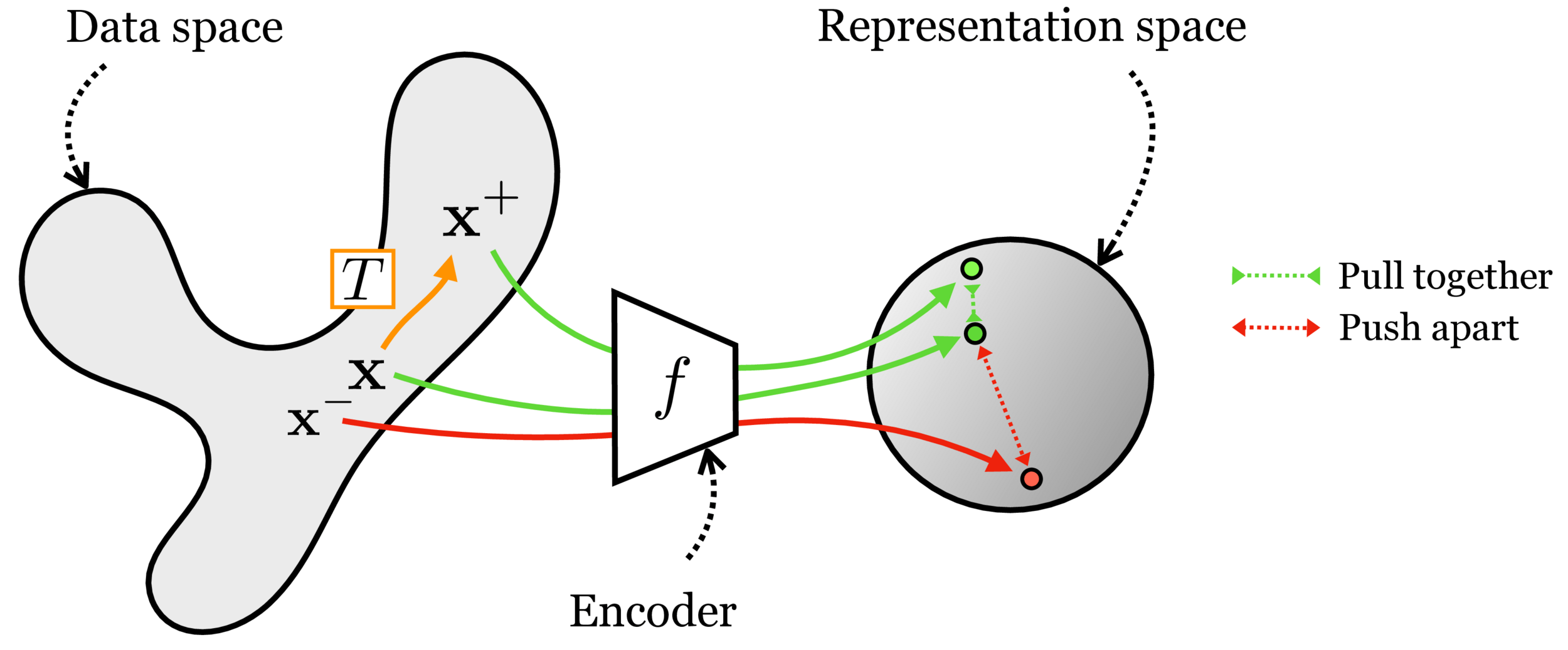

[Chen, Kornblith, Norouzi, Hinton, ICML 2020]
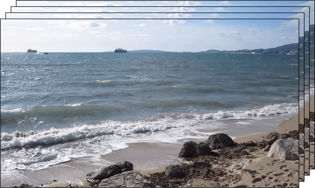
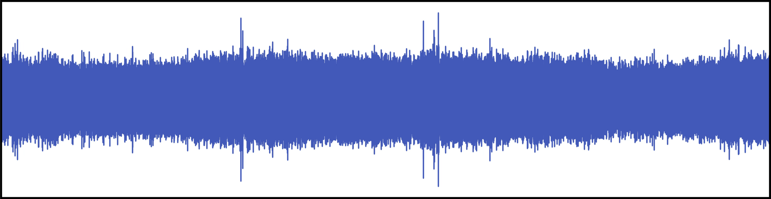
[Slide credit: Andrew Owens]
[Owens et al, Ambient Sound Provides Supervision for Visual Learning, ECCV 2016]
[Slide credit: Andrew Owens]
[Owens et al, Ambient Sound Provides Supervision for Visual Learning, ECCV 2016]
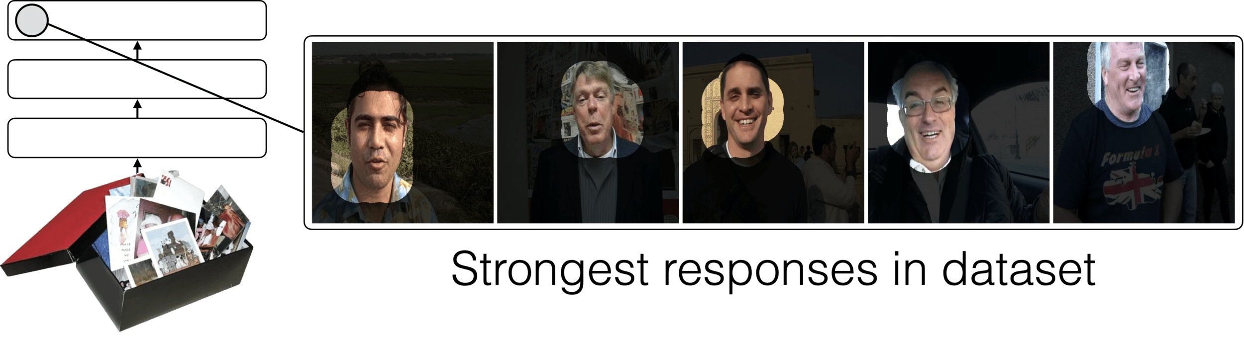
What did the model learn?
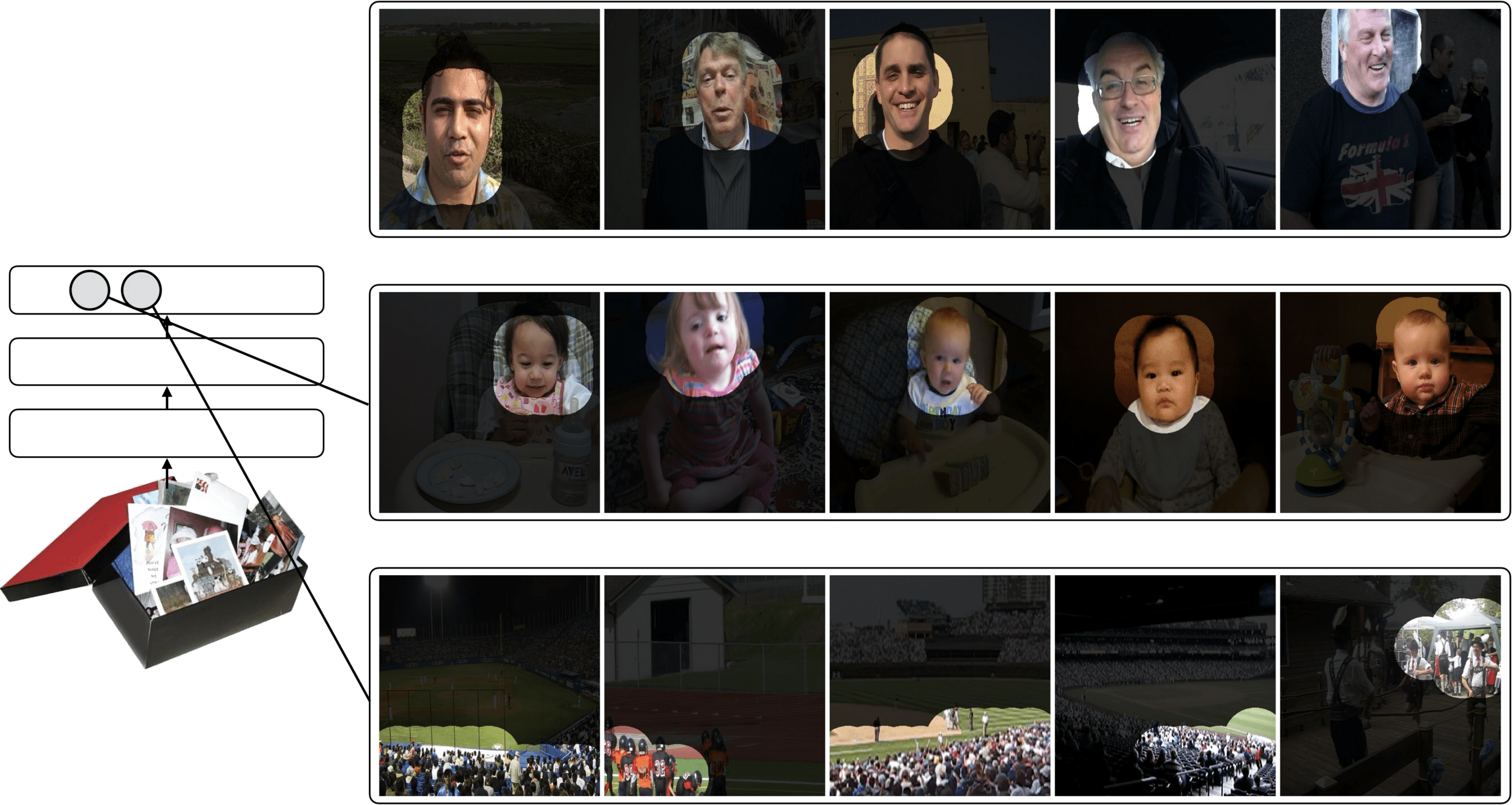
[Slide credit: Andrew Owens]
[Owens et al, Ambient Sound Provides Supervision for Visual Learning, ECCV 2016]
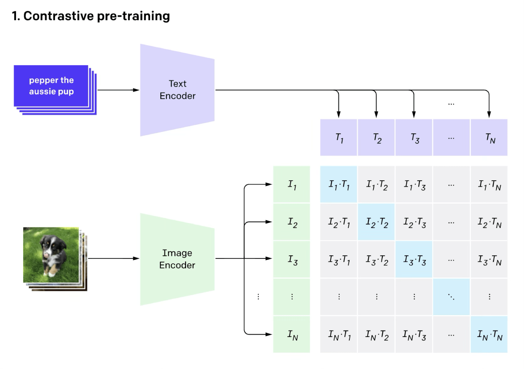
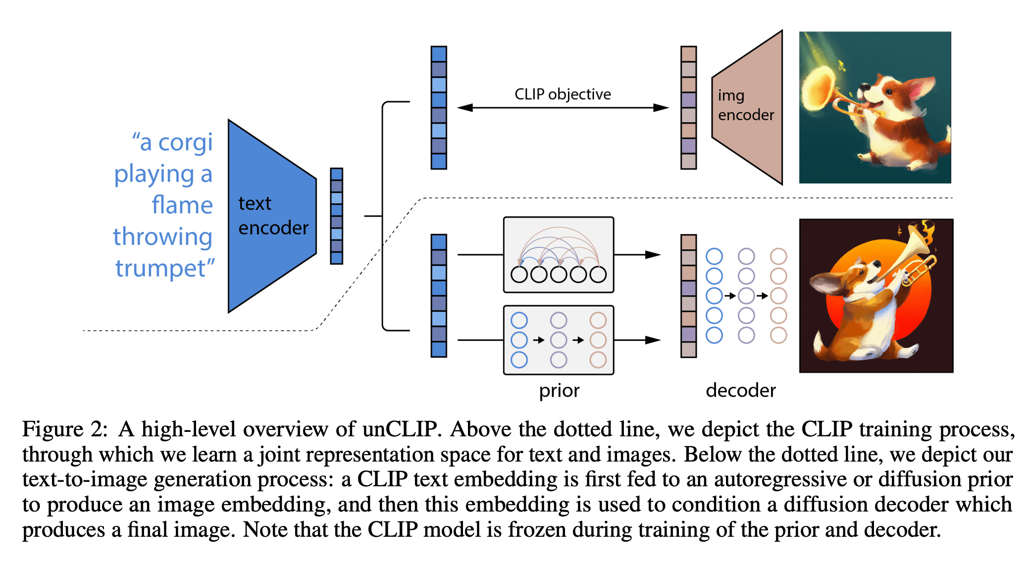
[https://arxiv.org/pdf/2204.06125.pdf]
DallE
A few other examples
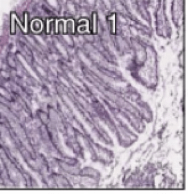
- learning to predict diagnosis, staging from histology slides different crops from the same slide can be used as positive examples, crops from different slides as negatives in contrastive training
- we can use clip-style association for learning to process medical records learning to associate parts of the record to their right complements
- we can take EEG signals and use different time segments from the same individual/session as positives pairs, different ones as negatives
- masked language modeling for biosequences (e.g., proteins)
- Etc.
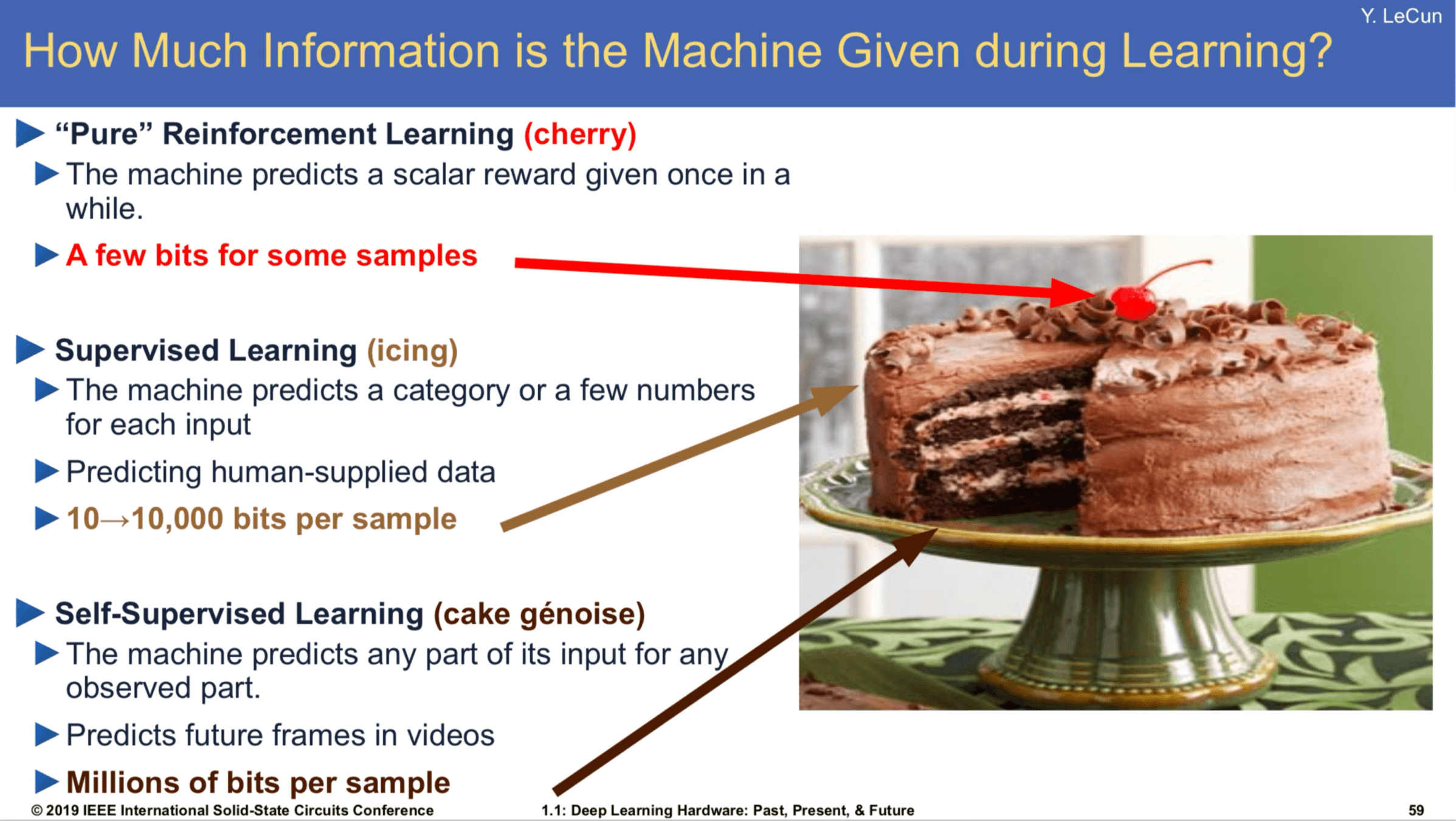
[Slide Credit: Yann LeCun]
Thanks!
We'd love to hear your thoughts.
Summary
- We looked at the mechanics of neural net last time. Today we see deep nets learn representations, just like our brains do.
- This is useful because representations transfer — they act as prior knowledge that enables quick learning on new tasks.
- Representations can also be learned without labels, e.g. as we do in unsupervised, or self-supervised learning. This is great since labels are expensive and limiting.
- Without labels there are many ways to learn representations. We saw today:
- representations as compressed codes, auto-encoder with bottleneck
- (representations that are shared across sensory modalities)
- (representations that are predictive of their context)
Outline
- Recap, neural networks mechanism
- Neural networks are representation learners
- Auto-encoder:
- Bottleneck
- Reconstruction
- Unsupervised learning
- (Some recent representation learning ideas)
- Clustering
(auto encoder slides adapted from Phillip Isola)
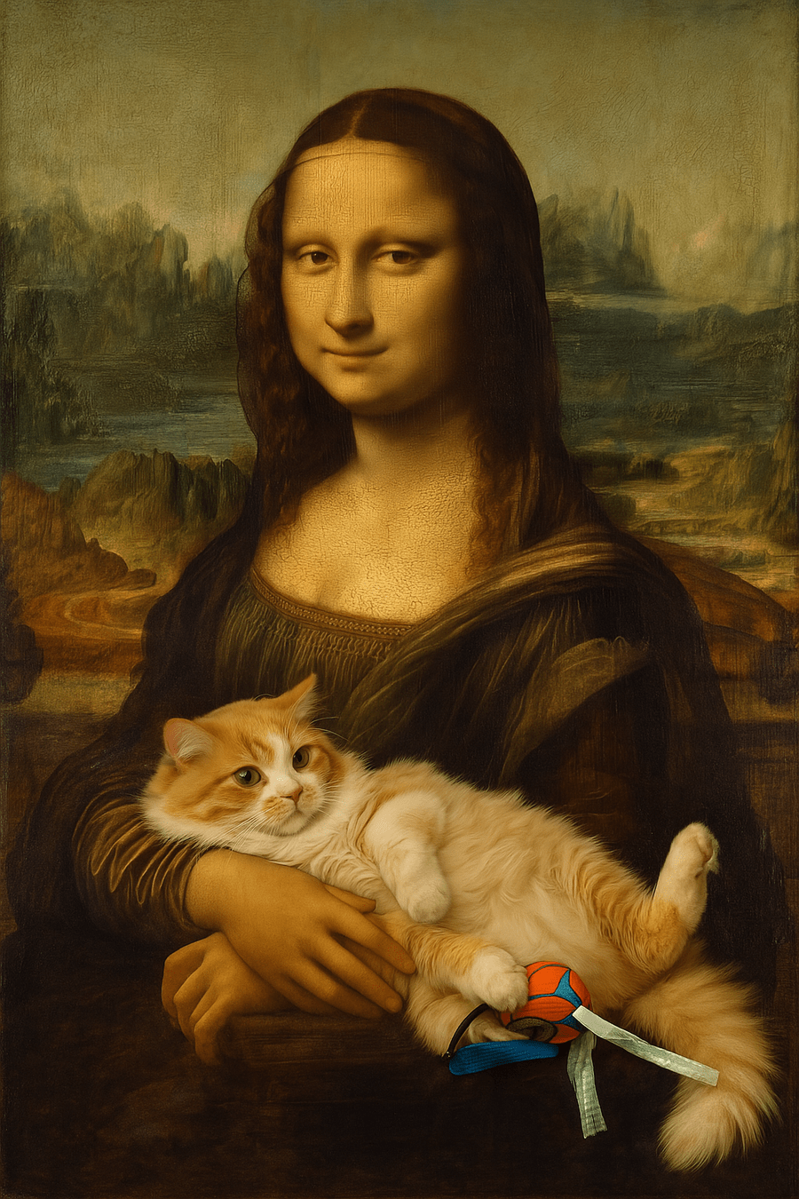
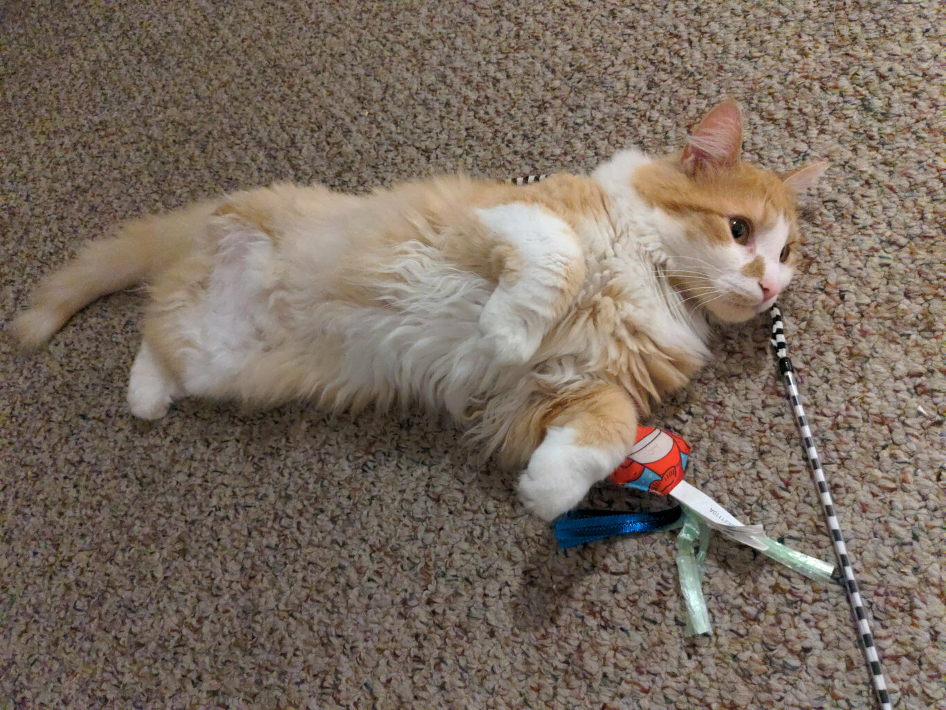
GPT 4o: multi-modal image generation
prompt: "make an image of Mona Lisa holding this cat"
[this cat is button]
Outline
- Recap, neural networks mechanism
- Neural networks are representation learners
- Auto-encoder:
- Bottleneck
- Reconstruction
- Unsupervised learning
- (Some recent representation learning ideas)
6.C011/C511 - ML for CS (Spring25) - Lecture 1 Representation Learning
By Shen Shen


