
Lecture 7: Reinforcement Learning (Actor-critic; variance reduction)
Shen Shen
April 23, 2025
2:30pm, Room 32-144
Modeling with Machine Learning for Computer Science

Outline
- Recap: Policy gradient
- RL challenges
- high variance
- sample complexity
- gradient update step-size issue
Policy Gradient Derivation
- We overload notation:
- Let \(\tau\) denote a state-action sequence: \(\tau=s_0, a_0, s_1, a_1, \ldots\)
- Let \(R(\tau)\) denote the sum of discounted rewards on \(\tau: R(\tau)=\sum_t \gamma^t R\left(s_t, a_t\right)\)
- W.l.o.g. assume \(R(\tau)\) is deterministic in \(\tau\)
- Let \(P(\tau ; \theta)\) denote the probability of trajectory \(\tau\) induced by \(\pi_\theta\)
- Let \(U(\theta)\) denote the objective: \(U(\theta)=\mathbb{E}\left[\sum_t \gamma^t R\left(s_t, a_t\right) \mid \pi_\theta\right]\)
- Our goal is to find \[\theta: \max _\theta U(\theta)=\max _\theta \sum_\tau P(\tau ; \theta) R(\tau)\]
Recap
Policy Gradient Derivation
Identity (quite useful in ML)
\(\begin{aligned} \nabla_\theta p_\theta(\tau) & =p_\theta(\tau) \frac{\nabla_\theta p_\theta(\tau)}{p_\theta(\tau)} \\ & =p_\theta(\tau) \nabla_\theta \log p_\theta(\tau)\end{aligned}\)
\(=\nabla_\theta \sum_\tau P(\tau ; \theta) R(\tau)\)
\(=\sum_\tau \nabla_\theta P(\tau ; \theta) R(\tau)\)
\(=\sum_\tau \frac{P(\tau ; \theta)}{P(\tau ; \theta)} \nabla_\theta P(\tau ; \theta) R(\tau)\)
\(=\sum_\tau P(\tau ; \theta) \frac{\nabla_\theta P(\tau ; \theta)}{P(\tau ; \theta)} R(\tau)\)
\(=\sum_\tau P(\tau ; \theta) \nabla_\theta \log P(\tau ; \theta) R(\tau)\)
\(\nabla_\theta U(\theta)\)
Recap
Policy Gradient Derivation
where \(P(\tau ; \theta)=\prod_{t=0} \underbrace{P\left(s_{t+1} \mid s_t, a_t\right)}_{\text {transition }} \cdot \underbrace{\left.\pi_\theta\left(a_t \mid s_t\right)\right]}_{\text {policy }}\)
\(=\sum_\tau P(\tau ; \theta) \nabla_\theta \log P(\tau ; \theta) R(\tau)\)
\(\nabla_\theta U(\theta)\)
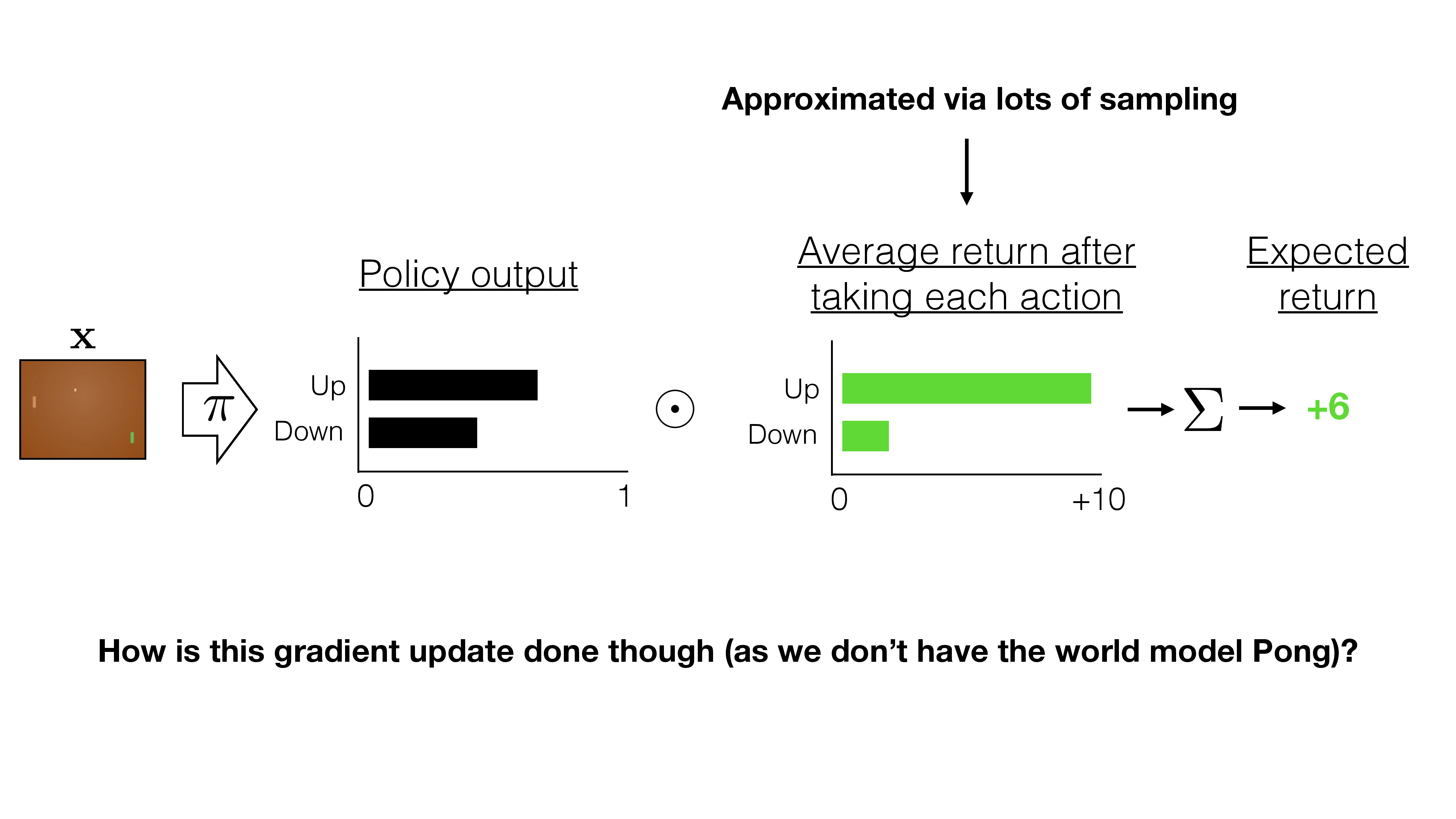
Transition is unknown....
Stuck?
Recap
Policy Gradient Derivation
\(=\sum_\tau P(\tau ; \theta) \nabla_\theta \log P(\tau ; \theta) R(\tau)\)
Approximate with the empirical (Monte-Carlo) estimate for \(m\) sample traj. under policy \(\pi_\theta\)
\(\nabla_\theta U(\theta) \approx \hat{g}=\frac{1}{m} \sum_{i=1}^m \nabla_\theta \log P\left(\tau^{(i)} ; \theta\right) R\left(\tau^{(i)}\right)\)
Valid even when:
- Reward function discontinuous and/or unknown
- Discrete state and/or action spaces
\(\nabla_\theta U(\theta)\)
Recap
Policy Gradient Derivation
where \(P(\tau ; \theta)=\prod_{t=0} \underbrace{P\left(s_{t+1} \mid s_t, a_t\right)}_{\text {transition }} \cdot \underbrace{\left.\pi_\theta\left(a_t \mid s_t\right)\right]}_{\text {policy }}\)
\(=\nabla_\theta \log [\prod_{t=0} \underbrace{P\left(s_{t+1} \mid s_t, a_t\right)}_{\text {transition }} \cdot \underbrace{\left.\pi_\theta\left(a_t \mid s_t\right)\right]}_{\text {policy }}\)
\(=\nabla_\theta\left[\sum_{t=0} \log P\left(s_{t+1} \mid s_t, a_t\right)+\sum_{t=0} \log \pi_\theta\left(a_t \mid s_t\right)\right]\)
\(=\nabla_\theta \sum_{t=0} \log \pi_\theta\left(a_t \mid s_t\right)\)
\(=\sum_{t=0} \underbrace{\nabla_\theta \log \pi_\theta\left(a_t \mid s_t\right)}_{\text {no transition model required, }}\)
\(\nabla_\theta \log P(\tau ; \theta)\)
\(\nabla_\theta U(\theta) \approx \hat{g}=\frac{1}{m} \sum_{i=1}^m \nabla_\theta \log P\left(\tau^{(i)} ; \theta\right) R\left(\tau^{(i)}\right)\)
Recap
Policy Gradient Derivation
\(=\sum_{t=0} \underbrace{\nabla_\theta \log \pi_\theta\left(a_t \mid s_t\right)}_{\text {no transition model required}}\)
\(\nabla_\theta \log P(\tau ; \theta)\)
\(\nabla_\theta U(\theta) \approx \hat{g}=\frac{1}{m} \sum_{i=1}^m \nabla_\theta \log P\left(\tau^{(i)} ; \theta\right) R\left(\tau^{(i)}\right)\)
The following expression provides us with an unbiased estimate of the gradient, and we can compute it without access to the transition model:

Unbiased estimator \(\mathrm{E}[\hat{g}]=\nabla_\theta U(\theta)\), but very noisy.
where
Recap
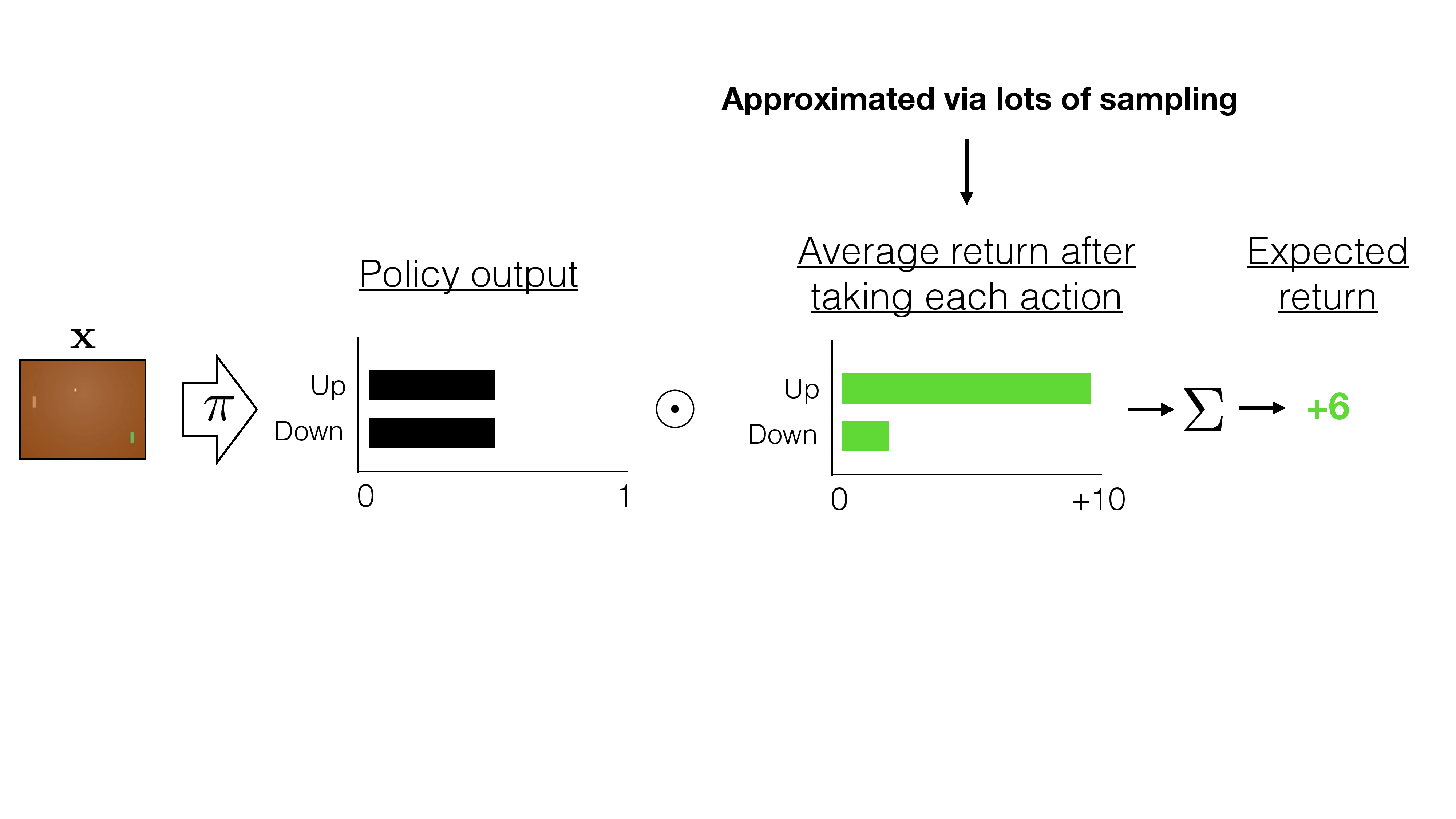
\(=\sum_\tau P(\tau ; \theta) R(\tau)\)
\(U(\theta)\)
\(\approx \hat{g} = \frac{1}{m}\sum_{i=1}^{m}\left(\sum_{t=0}\nabla_\theta \log \pi_\theta(a_t^{(i)}\mid s_t^{(i)})\right)R(\tau^{(i)})\)
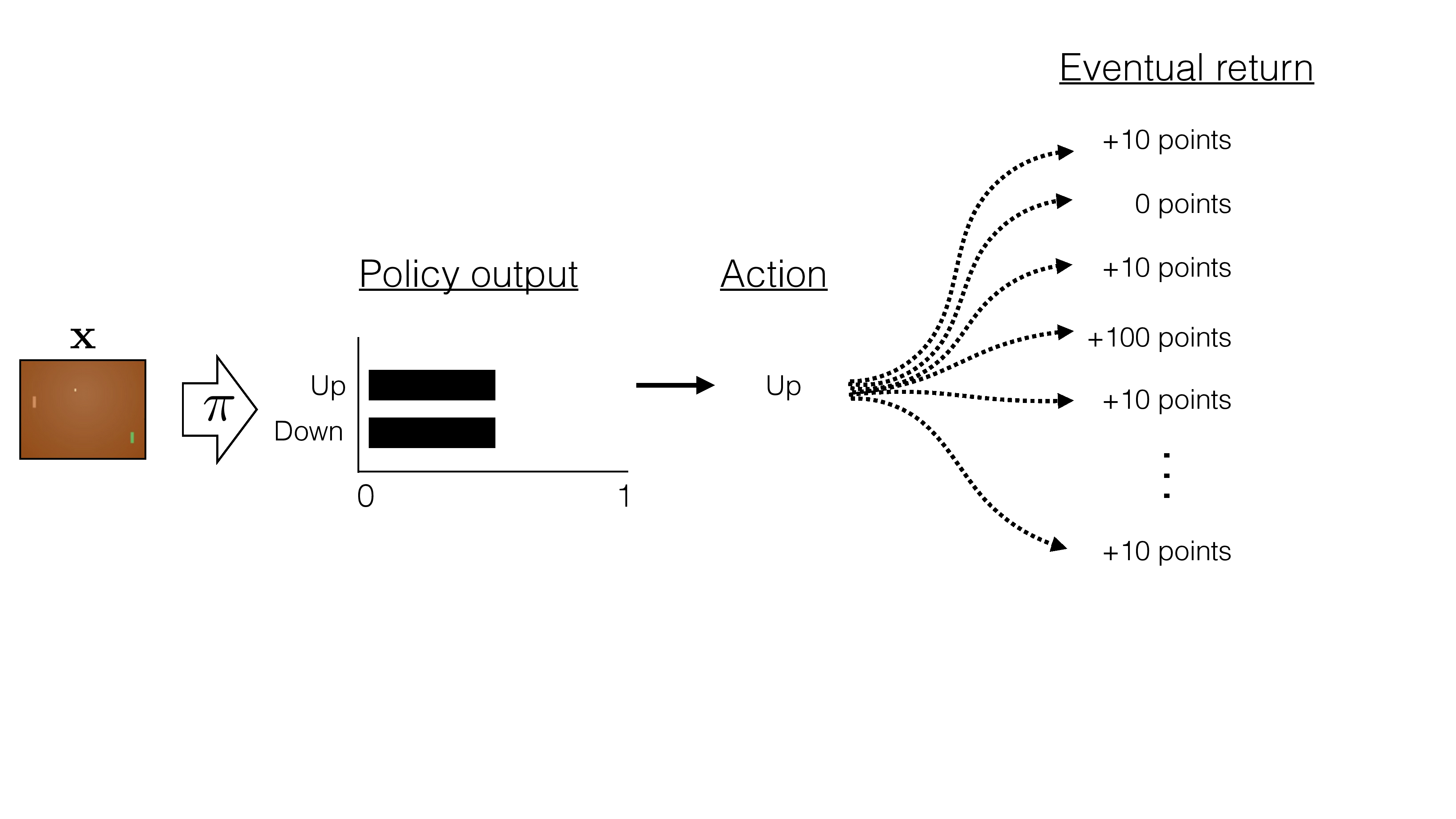
This policy gradient estimator typically has high variance, due to:
- Trajectory-Level Monte Carlo Sampling
- Single-trajectory randomness: The gradient estimator \(\hat{g}\) depends on averaging the returns from a finite set of \(m\) trajectories.
- Each trajectory \(\tau^{(i)}\) is sampled from the policy \(\pi_\theta\), making it inherently stochastic and subject to large fluctuations.
\(=\frac{1}{m} \sum_{i=1}^m \nabla_\theta \log P\left(\tau^{(i)} ; \theta\right) R\left(\tau^{(i)}\right)\)
\(\nabla_\theta U(\theta)\)
\(=\sum_\tau P(\tau ; \theta) R(\tau)\)
\(U(\theta)\)
\(\nabla_\theta U(\theta) \approx \hat{g} = \frac{1}{m}\sum_{i=1}^{m}\left(\sum_{t=0}\nabla_\theta \log \pi_\theta(a_t^{(i)}\mid s_t^{(i)})\right)R(\tau^{(i)})\)
This policy gradient estimator typically has high variance, due to:
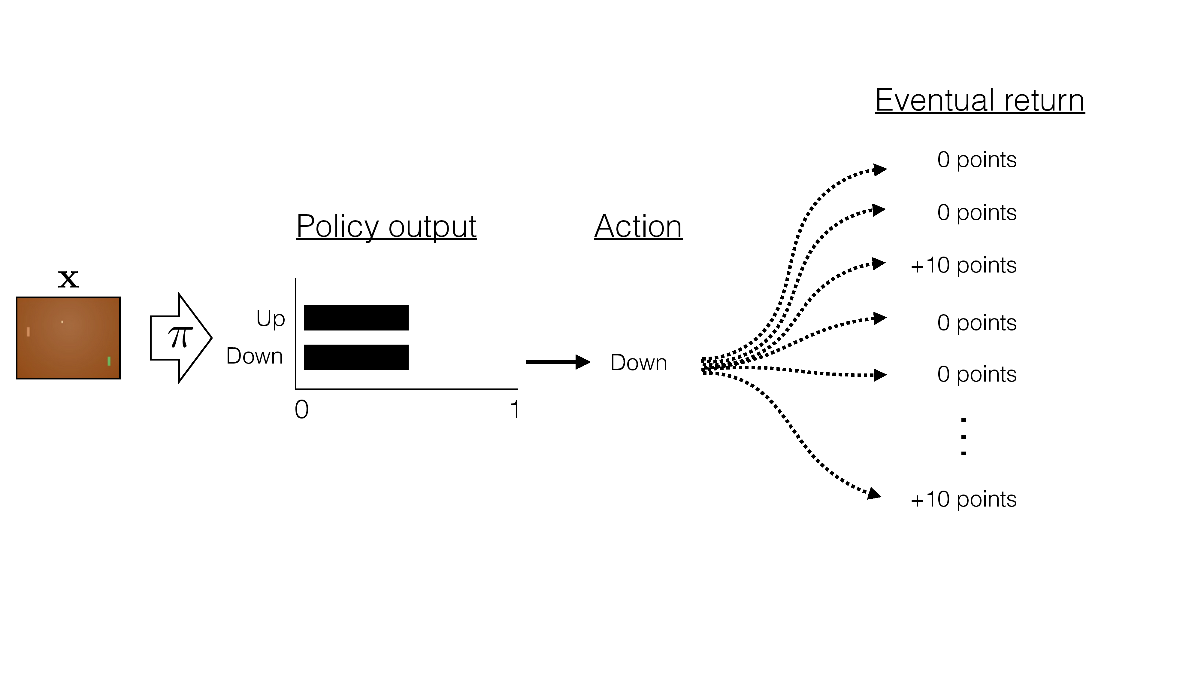
- High Variance of Return \(R(\tau^{(i)})\)
- Cumulative rewards: The return \(R(\tau^{(i)})\) is the sum of all rewards along the trajectory. A slight variation in early steps can produce large differences in total returns.
- Sparse or delayed rewards: When rewards are sparse or rare, returns can fluctuate drastically—some trajectories yield high rewards, others yield zero.
\(=\sum_\tau P(\tau ; \theta) R(\tau)\)
\(U(\theta)\)
\(\nabla_\theta U(\theta) \approx \hat{g} = \frac{1}{m}\sum_{i=1}^{m}\left(\sum_{t=0}\nabla_\theta \log \pi_\theta(a_t^{(i)}\mid s_t^{(i)})\right)R(\tau^{(i)})\)
This policy gradient estimator typically has high variance, due to:
- Noisy Gradient via \(\nabla_\theta \log \pi_\theta(a_t \mid s_t)\)
- Log probability gradients: The term \(\nabla_\theta \log \pi_\theta(a_t^{(i)} \mid s_t^{(i)})\) can fluctuate significantly, as small parameter changes affect action probabilities greatly, especially with neural-network policies.
- Multiplicative variance amplification: Since the return \(R(\tau^{(i)})\) multiplies this gradient, any small variance in the log-policy gradients is amplified by large or variable returns.
\(=\sum_\tau P(\tau ; \theta) R(\tau)\)
\(U(\theta)\)
\(\nabla_\theta U(\theta) \approx \hat{g} = \frac{1}{m}\sum_{i=1}^{m}\left(\sum_{t=0}\nabla_\theta \log \pi_\theta(a_t^{(i)}\mid s_t^{(i)})\right)R(\tau^{(i)})\)
This policy gradient estimator typically has high variance, due to:
- Credit Assignment Problem
- Long-horizon dependencies: Rewards received late in a trajectory affect all preceding time-step gradient updates equally, regardless of which actions truly contributed. This leads to noisy and uncertain gradient signals for early actions.
- Poor causality: The gradient estimator does not explicitly distinguish between actions genuinely contributing to a high return and those irrelevant to it.
\(=\sum_\tau P(\tau ; \theta) R(\tau)\)
\(U(\theta)\)
\(\nabla_\theta U(\theta) \approx \hat{g} = \frac{1}{m}\sum_{i=1}^{m}\left(\sum_{t=0}\nabla_\theta \log \pi_\theta(a_t^{(i)}\mid s_t^{(i)})\right)R(\tau^{(i)})\)
This policy gradient estimator typically has high variance, due to:
- Limited Sample Size (\(m\) small)
- Finite-sample estimation: Typically, only a limited number \(m\) of trajectories are sampled. Small sample sizes mean high sampling variability, thus high estimator variance.
- Expensive sampling: Generating trajectories is computationally expensive, limiting practical trajectory counts and exacerbating variance.
Variance reduction:
- Getting more sample trajectories (sometimes infeasible)
- Temporal structure
- Subtracting a constant baseline \(b\)
\(\hat{g}=\frac{1}{m} \sum_{i=1}^m \nabla_\theta \log P\left(\tau^{(i)} ; \theta\right)\left(R\left(\tau^{(i)}\right)\right)\)
\(=\frac{1}{m} \sum_{i=1}^m\left(\sum_{t=0}^{h-1} \nabla_\theta \log \pi_\theta\left(a_t^{(i)} \mid s_t^{(i)}\right)\right)\left(\sum_{t=0}^{h-1} R\left(s_t^{(i)}, a_t^{(i)}\right)\right)\)
\(=\frac{1}{m} \sum_{i=1}^m\left(\sum_{t=0}^{I I-1} \nabla_\theta \log \pi_\theta\left(a_t^{(i)} \mid s_t^{(i)}\right)\left[\left(\sum_{k=0}^{t-1} R\left(s_k^{(i)}, a_k^{(i)}\right)\right)+\left(\sum_{k=t}^{h-1} R\left(s_k^{(i)}, a_k^{(i)}\right)\right)\right]\right)\)
[Policy Gradient Theorem: Sutton et al 1999; GPOMDP: Bartlett & Baxter, 2001; Survey: Peters & Schaal, 2006]
Removing terms that don't depend on current action can lower variance:
\(\frac{1}{m} \sum_{i=1}^m \sum_{t=0}^{h-1} \nabla_\theta \log \pi_\theta\left(a_t^{(i)} \mid s_t^{(i)}\right)\left(\sum_{k=t}^{h-1} R\left(s_k^{(i)}, a_k^{(i)}\right)\right)\)
Temporal structure
Variance reduction:
- Subtracting a constant baseline \(b:\)
\(\nabla U(\theta) \approx \hat{g}=\frac{1}{m} \sum_{i=1}^m \nabla_\theta \log P\left(\tau^{(i)} ; \theta\right)\left(R\left(\tau^{(i)}\right)-b\right)\)
[Williams, REINFORCE paper, 1992]
- Still unbiased, despite the additional term
\[\frac{1}{m} \sum_{i=1}^m \nabla_\theta \log P\left(\tau^{(i)} ; \theta\right)(-b)\]
- with good choice of \(b,\) can reduce variance of \(\nabla U(\theta)\)
\(\nabla U(\theta) \approx \hat{g}=\frac{1}{m} \sum_{i=1}^m \nabla_\theta \log P\left(\tau^{(i)} ; \theta\right)\left(R\left(\tau^{(i)}\right)-b\right)\)
\(\begin{aligned} & \mathbb{E}\left[\nabla_\theta \log P(\tau ; \theta) b\right] \\ & =\sum_\tau P(\tau ; \theta) \nabla_\theta \log P(\tau ; \theta) b \\ & =\sum_\tau P(\tau ; \theta) \frac{\nabla_\theta P(\tau ; \theta)}{P(\tau ; \theta)} b \\ & =\sum_\tau \nabla_\theta P(\tau ; \theta) b\end{aligned}\)
\(=\nabla_\theta\left(\sum_\tau P(\tau) b\right)=b \nabla_\theta\left(\sum_\tau P(\tau)\right)=b \times 0\)
[Williams, REINFORCE paper, 1992]
❓ Why still unbiased despite the additional term
\[\frac{1}{m} \sum_{i=1}^m \nabla_\theta \log P\left(\tau^{(i)} ; \theta\right)(-b)\]
Variance reduction:
- Getting more sample trajectories (sometimes infeasible)
- Subtracting a constant baseline \(b:\)
\(\nabla U(\theta) \approx \hat{g}=\frac{1}{m} \sum_{i=1}^m \nabla_\theta \log P\left(\tau^{(i)} ; \theta\right)\left(R\left(\tau^{(i)}\right)-b\right)\)
[Williams, REINFORCE paper, 1992]
✅ Still unbiased, despite the additional term
\[\frac{1}{m} \sum_{i=1}^m \nabla_\theta \log P\left(\tau^{(i)} ; \theta\right)(-b)\]
❓with good choice of \(b,\) can reduce variance of \(\nabla U(\theta)\)
Control Variates
- The main idea is to reduce variance in the estimate of an expectation.
- Suppose we want to estimate: \[\mu = \mathbb{E}[X]\] where \(X\) is some random variable.
- We introduce another random variable \(Y\) (the control variate), with a known expectation \(\mathbb{E}[Y] = \nu\), and importantly, \(Y\) is correlated to \(X\).
- Estimator \(X-Y+\nu\) has variance \[\operatorname{Var}(X-Y)=\operatorname{Var}(X)+\operatorname{Var}(Y)-2 \operatorname{Cov}(X, Y)\]
We can also define a new estimator: \(X’ = X - \alpha(Y - \nu)\) where \(\alpha\) can be chosen optimally to minimize variance.
Control variates in RL
\(\nabla U(\theta) \approx \hat{g}=\frac{1}{m} \sum_{i=1}^m \nabla_\theta \log P\left(\tau^{(i)} ; \theta\right)\left(R\left(\tau^{(i)}\right)-b\right)\)
- What's a good baseline \(b\) candidate?
- state-value function \( V^\pi(s) \)) from rewards
- \(b=\frac{1}{m} \sum_{i=1}^m R\left(\tau^{(i)}\right)\)
- Estimated state-dependent value functions: \(b\left(s_t\right)=\hat{V}^\pi\left(s_t\right)\)
\(\nabla U(\theta) \approx \hat{g}=\frac{1}{m} \sum_{i=1}^m \nabla_\theta \log P\left(\tau^{(i)} ; \theta\right)\left(R\left(\tau^{(i)}\right)-\hat{V}^\pi(s)\right)\)
[Greensmith, Bartlett, Baxter, JMLR 2004 for variance reduction techniques.]
advantage function
\(-b\)
instead of increase the likelihood of all "winning" games, increase the likelihood of "better than average score" games
\(-b\)
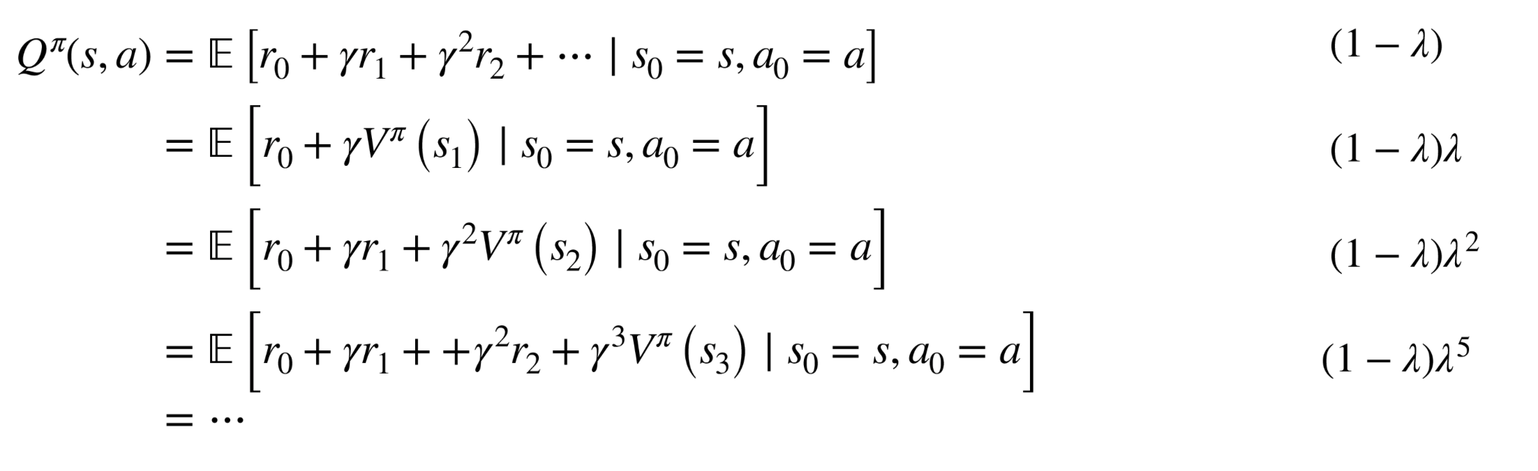
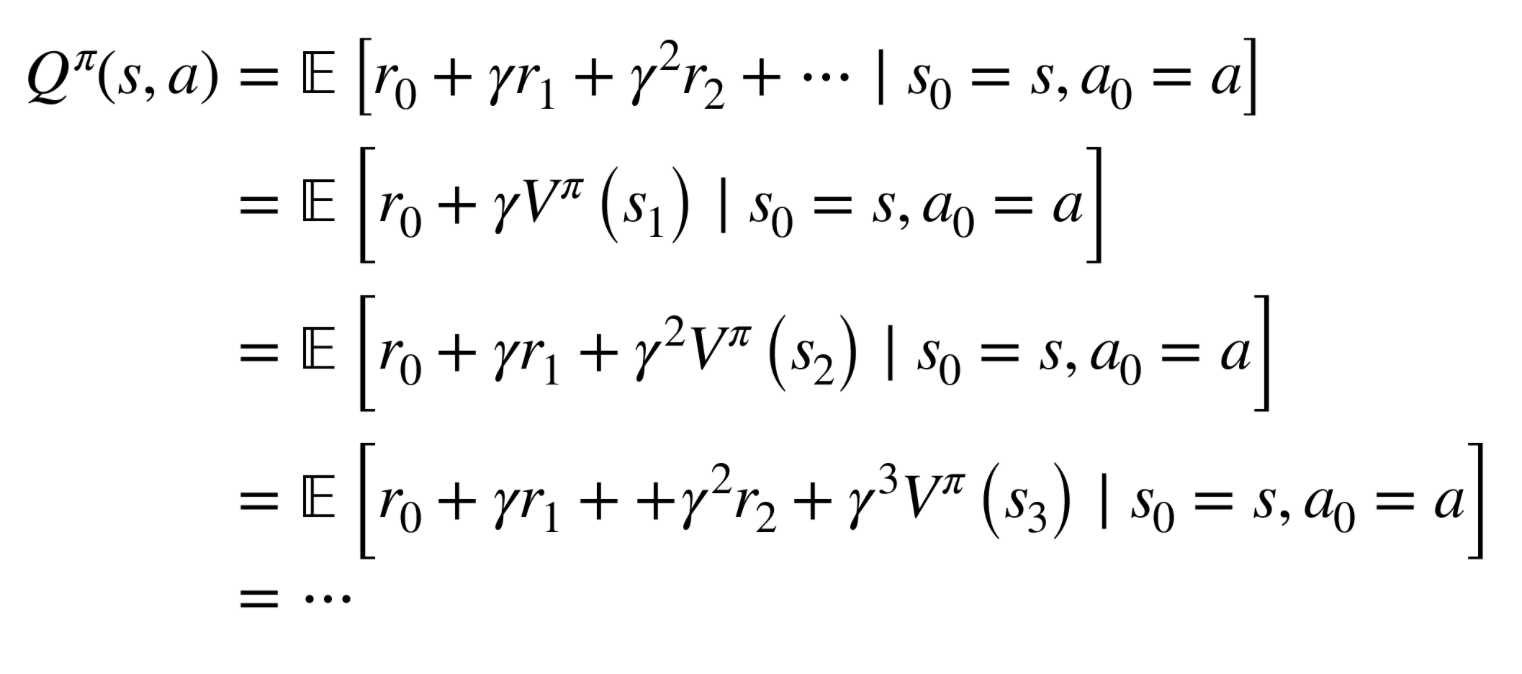
How to estimate \(V^\pi\)?
- Again, Monte Carlo estimate \(b\left(s_t\right)=\mathbb{E}\left[r_t+r_{t+1}+r_{t+2}+\ldots+r_{H-1}\right]=V^\pi\left(s_t\right)\)
-
Or, collect \(\tau_1, \ldots, \tau_m\), and regress against empirical return: \(\phi_{i+1} \leftarrow \underset{\phi}{\arg \min } \frac{1}{m} \sum_{i=1}^m \sum_{t=0}^{H-1}\left(V_\phi^\pi\left(s_t^{(i)}\right)-\left(\sum_{k=t}^{H-1} R\left(s_k^{(i)}, u_k^{(i)}\right)\right)\right)^2\)
-
Or, similar to fitted Q-learning, do fitted V-learning: \(\phi_{i+1} \leftarrow \min _\phi \sum_{\left(s, u, s^{\prime}, r\right)}\left\|r+V_{\phi_i}^\pi\left(s^{\prime}\right)-V_\phi(s)\right\|_2^2\)
[Greensmith, Bartlett, Baxter, JMLR 2004 for variance reduction techniques.]
How to estimate advatange?
(GAE) [Schulman et al, ICLR 2016]
TD(lambda) / eligibility traces [Sutton and Barto, 1990]
- \(\hat{Q}:\) lambda exponentially weighted average of all the above
- Advantage estimate then \(\hat{A}=\hat{Q}-\hat{V}\)
How to estimate advatange?
[Async Advantage Actor Critic (A3C) [Mnih et al, 2016]
- \(\hat{Q}\) : one of the above choices (e.g. k=5 step lookahead)
- Advantage estimate then \(\hat{A}=\hat{Q}-\hat{V}\)
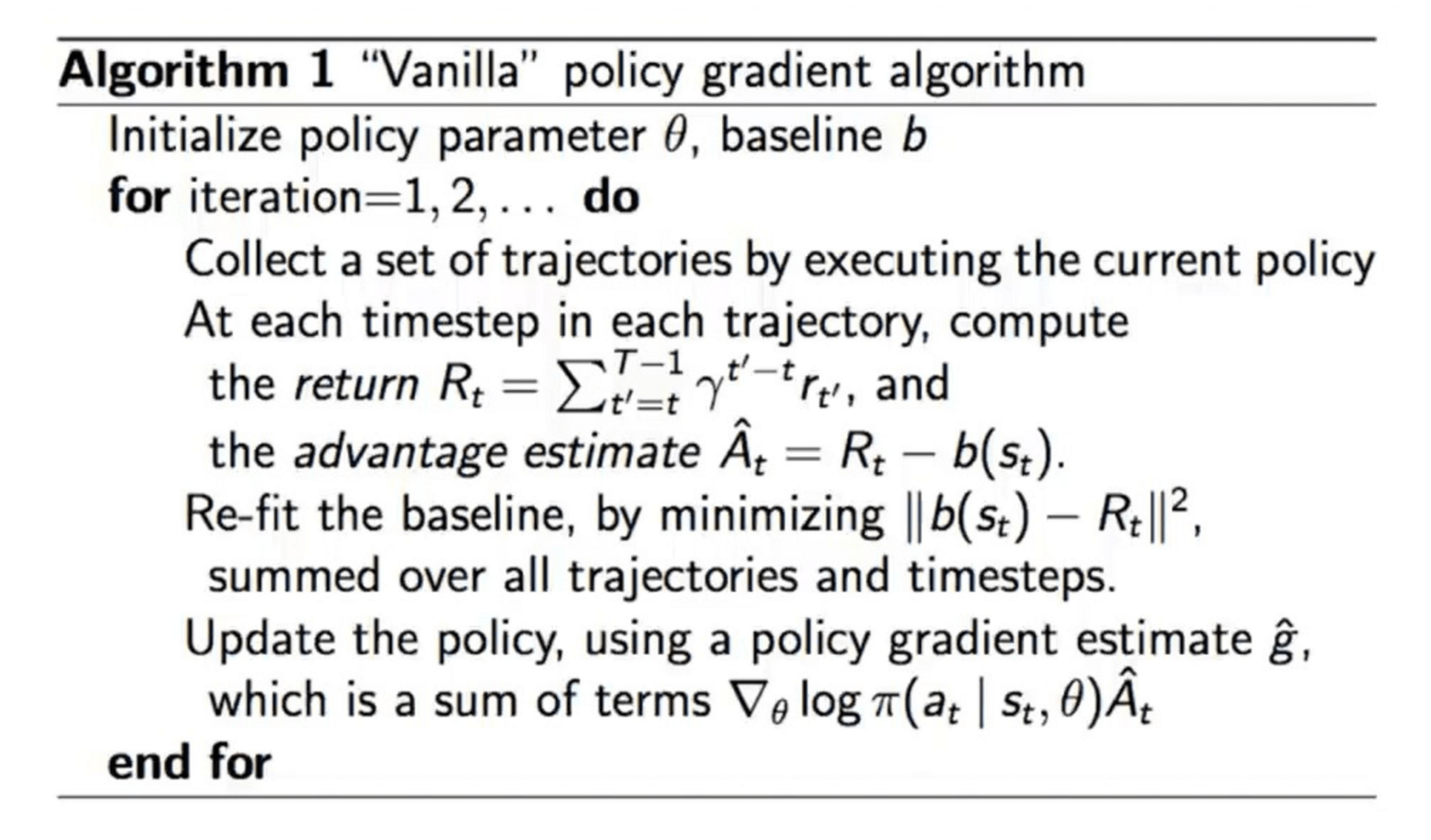
Actor-critic method
[Williams, REINFORCE paper, 1992]
actor
critic
Vanilla policy gradient/REINFORCE: step-sizing issue
- Step-sizes is worth tuning even in pure SGD under supervised learning.
- In policy gradient, bad step-sizes can have worse "chain effect":
- Step too far, may lead to terrible policy
- Next mini-batch: terrible data collected (with e.g. no reward signal; so no "correction")
- Not clear how to recover
- Intuitively, too big of a distributional shift
- Coupled with unknown dynamics/transition, good step-sizing is hard a-priori
Trust region policy optimization (TRPO)
- Interpretation of the objective via importance sampling (next slide)
- Interpretation of the constraint via distributional shift
- Can solve approximately via conjugate gradient method (using linear approx. of the objective and quadratic approx. of the KL)
\(\max L(\pi)=\mathbb{E}_{\pi \text { old }}\left[\frac{\pi(a \mid s)}{\pi_{\mathrm{old}}(a \mid s)} A^\pi_{old}\right.\)\(\left.(s, a)\right]\)
Constraint: \(\quad \mathbb{E}_{\pi_{\text {old }}}\left[K L\left(\pi \mid \pi_{\text {old }}\right)\right] \leq \epsilon\)
importance sampling
\(\mathbb{E}_{x \sim q}\left[\frac{p(x)}{q(x)} f(x)\right]=\mathbb{E}_{x \sim p}[f(x)]\)
\(U(\theta)=\mathbb{E}_{\tau \sim \theta} \mathrm{old}\left[\frac{P(\tau \mid \theta)}{P\left(\tau \mid \theta_{\mathrm{old}}\right)} R(\tau)\right]\)
\(=\mathbb{E}_{\tau \sim \theta_{\text {old }}}\left[\frac{\pi(\tau \mid \theta)}{\pi\left(\tau \mid \theta_{\text {old }}\right)} R(\tau)\right]\)
\(\nabla_\theta U(\theta)=\mathbb{E}_{\tau \sim \theta} \text { old }\left[\frac{\nabla_\theta P(\tau \mid \theta)}{P\left(\tau \mid \theta_{\text {old }}\right)} R(\tau)\right]\)
[Tang and Abbeel, On a Connection between Importance Sampling and the Likelihood Ratio Policy Gradient, 2011]
- Estimate both the utilities (objective) and policy gradient under new policy
- by using trajectories under old policy
- helps sample complexity, but increases variance actually (another tradeoff)
[Tang and Abbeel, On a Connection between Importance Sampling and the Likelihood Ratio Policy Gradient, 2011]
TRPO
\(\max L(\pi)=\mathbb{E}_{\pi \text { old }}\left[\frac{\pi(a \mid s)}{\pi_{\mathrm{old}}(a \mid s)} A^\pi_{old}\right.\)\(\left.(s, a)\right]\)
Constraint: \(\quad \mathbb{E}_{\pi_{\text {old }}}\left[K L\left(\pi \mid \pi_{\text {old }}\right)\right] \leq \epsilon\)
\(\max \mathbb{E}_{\pi \text { old }}\left[\frac{\pi(a \mid s)}{\pi_{\mathrm{old}}(a \mid s)} A^\pi_{old}\right.\)\(\left.(s, a)\right]\)
\(-\beta\left(\mathbb{E}_t\left[\operatorname{KL}\left(\pi_{o l d} \mid \pi\right)\right]-\delta\right)\)
Proximal Policy Optimization (PPO, v1)
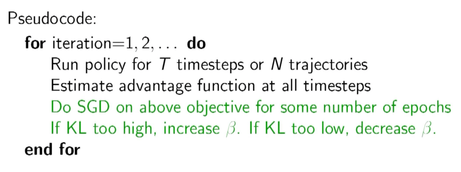
Proximal Policy Optimization (PPO, v2)
Recall the objective:
\(\hat{\mathbb{E}}_t\left[\frac{\pi_\theta\left(a_t \mid s_t\right)}{\pi_\theta \text { old }}{ }^{\left(a_t \mid s_t\right)} \hat{A}_t\right]\)
\(=\hat{\mathbb{E}}_t\left[\rho_t(\theta) \hat{A}_t\right]\)
A pwer bound of the above:
\(L^{C L I P}(\theta)=\hat{\mathbb{E}}_t\left[\min \left(\rho_t(\theta) \hat{A}_{t<0}, \operatorname{clip}\left(\rho_t(\theta), 1-\epsilon, 1+\epsilon\right) \hat{A}_t\right)\right]\)
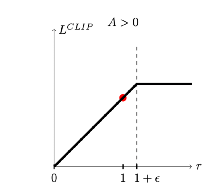
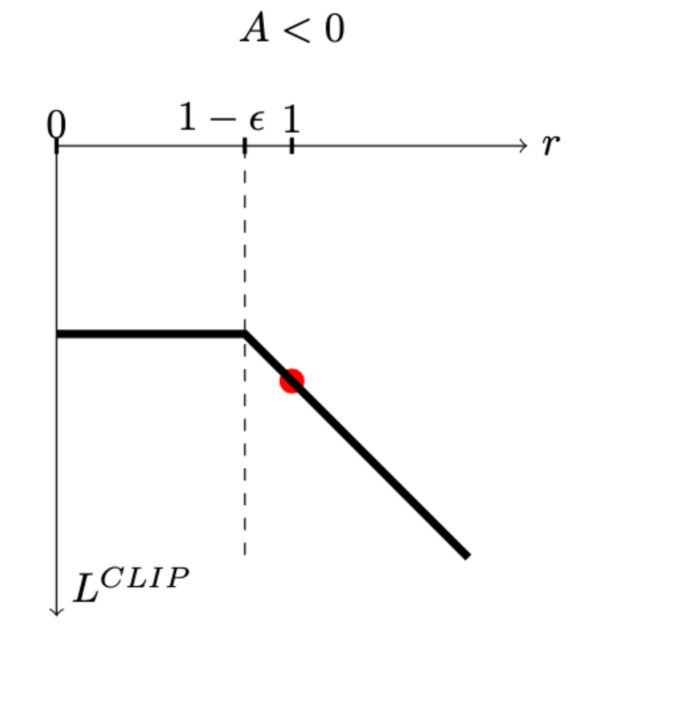
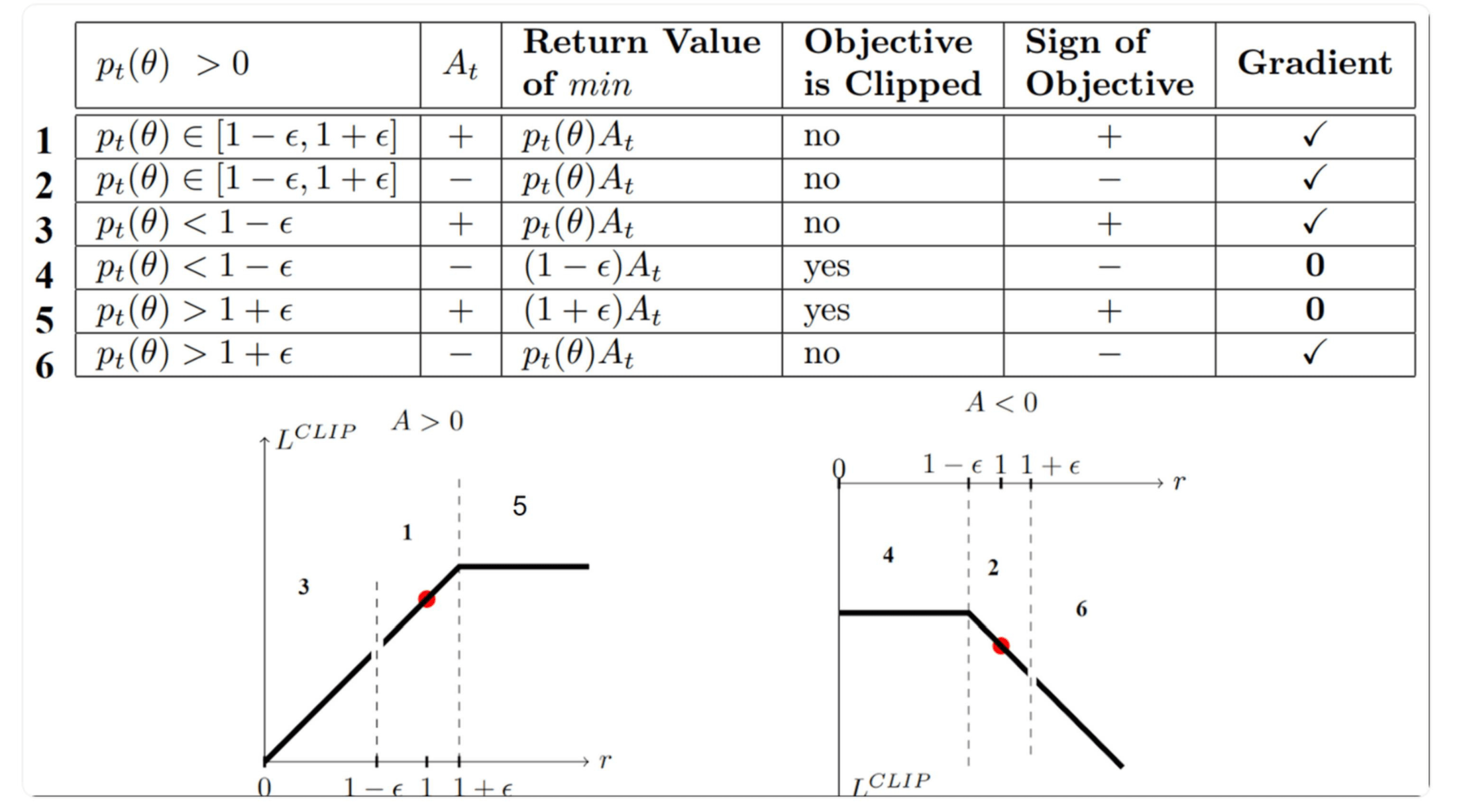
[table credit: Daniel Bick]
- The main loss \(L_t(\theta)=\min \left(r_t(\theta) \hat{A}_t, \operatorname{clip}\left(r_t(\theta)\right), 1-\epsilon, 1+\epsilon\right) \hat{A}_t\)
- Advantage estimate based on truncated GAE
- Adding an entropy term
Beyond what we covered
- POMDP
- Inverse RL
- Apprenticeship learning
- Behavioral cloning (Data Augmentation, a.k.a. DAgger)
- Transfer learning (sim to real)
- Domain randomization
- Multi-task learning
- Curriculum learning
- Hierarchical RL
- Safe/verifiable RL
- Multi-agent RL
- Offline RL
- Rewards shaping
- Fairness, ethical, explainable AI (value alignment)
Thanks!
We'd love to hear your thoughts.
Variance Reduction Achieved
- With the optimal control variate estimator \(X'\): \[\mathrm{Var}(X') = \mathrm{Var}(X - 0.8(Y - 1)).\]
- Expanding explicitly: \[\mathrm{Var}(X') = \mathrm{Var}(X - 0.8(X+\varepsilon - 1)) = \mathrm{Var}(0.2X - 0.8\varepsilon) = (0.2^2)\mathrm{Var}(X) + (-0.8^2)\mathrm{Var}(\varepsilon) = (0.04)(4) + (0.64)(1)= 0.16 + 0.64 = 0.8.\]
- Thus, we reduced the variance significantly: \( 4 \rightarrow 0.8 \) (5× improvement).
6.C011/C511 - ML for CS (Spring25) - Lecture 7 - Reinforcement Learning III (Actor-critic; variance reduction)
By Shen Shen


