Characterising the Variability of the Black Hole at the Centre of our Galaxy using Multi-Output Gaussian Processes
Shih Ching Fu
shihching.fu@postgrad.curtin.edu.au
Supervisors:
Dr Arash Bahramian, Dr Aloke Phatak,
Dr James Miller-Jones, Dr Suman Rakshit

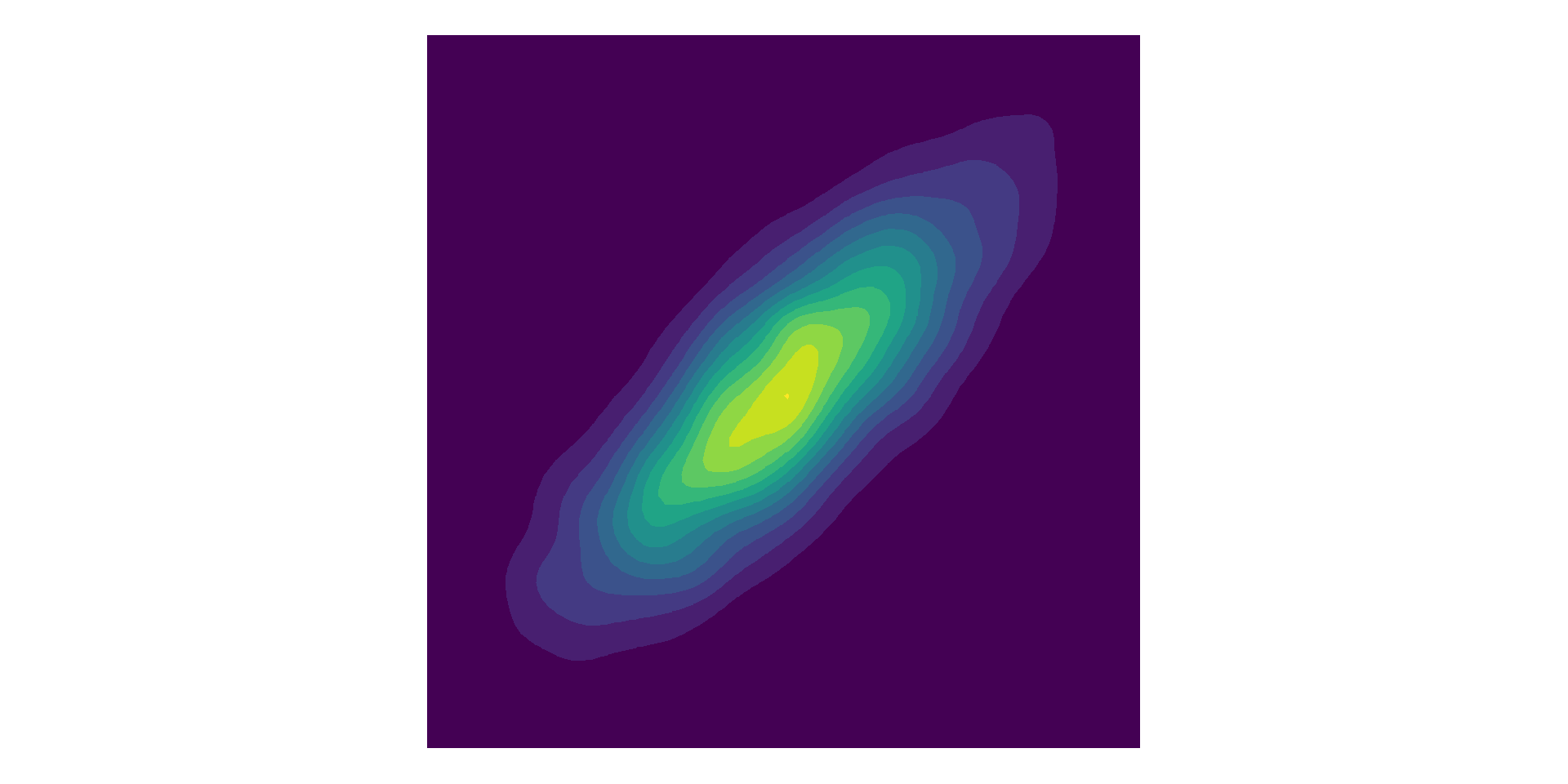
Sagittarius A* (Sgr A*)
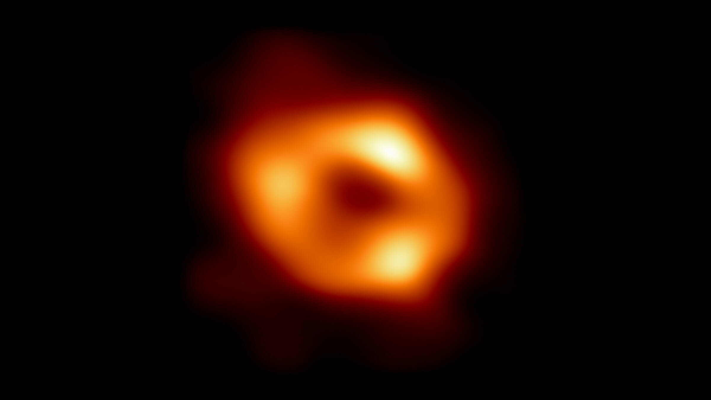
- Supermassive Black Hole (SMBH) at the centre of the Milky Way.
- 4 million solar masses.
- ~27,000 ly from Earth
- Image created from observations taken in 2017 by the Event Horizon Telesope (EHT) Collaboration.
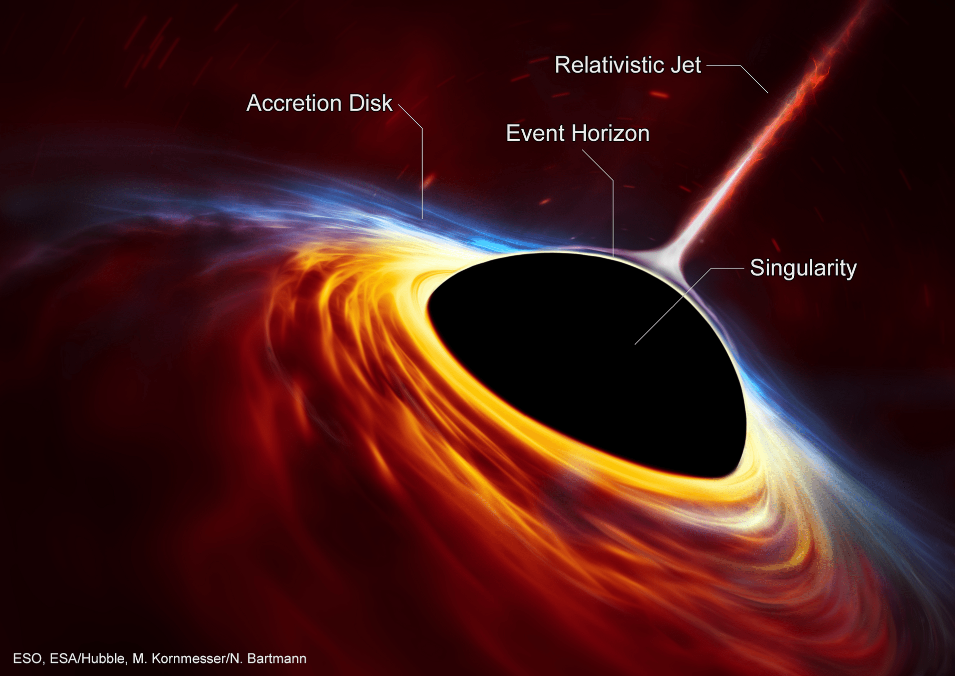
Anatomy of a Black Hole
Time domain astronomy
- Estimate the characteristic timescales of the variability in the black hole emissions.
- Characterise the relationship between emissions of different wavelengths, e.g, time delay between bands.
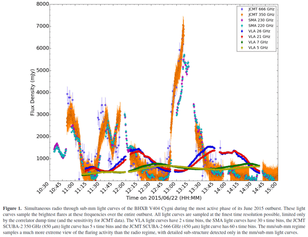
Credit: Tetarenko et al. (2017)
Black hole X-ray binary
V404 Cygni
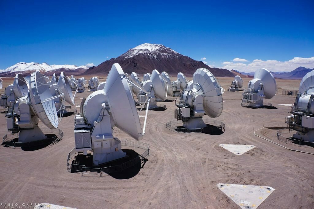
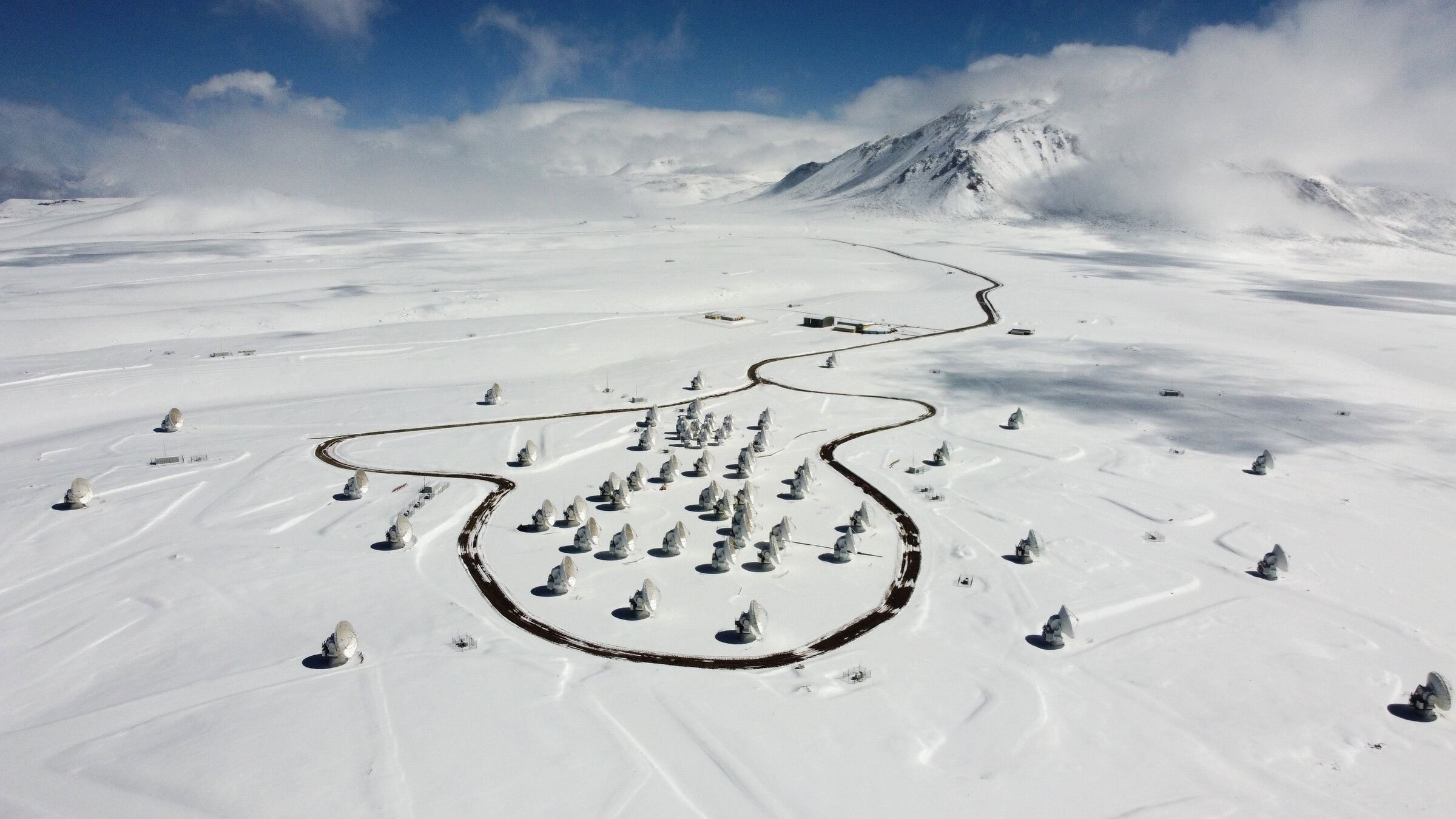
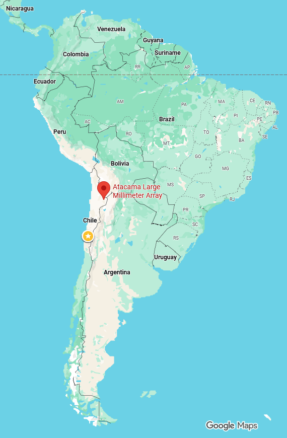
Atacama Large Millimeter Array (ALMA)
- Chilean Atacama Desert at 5000m elevation.
- 66 high-precision dish antennas: 54 x 12m and 12 x 7m across.
- Radio and infrared.
- Member site of EHT Collaboration.
Credit: NRAO/AUI/NSF
Credit: ALMA (ESO/NAOH/NRAO)
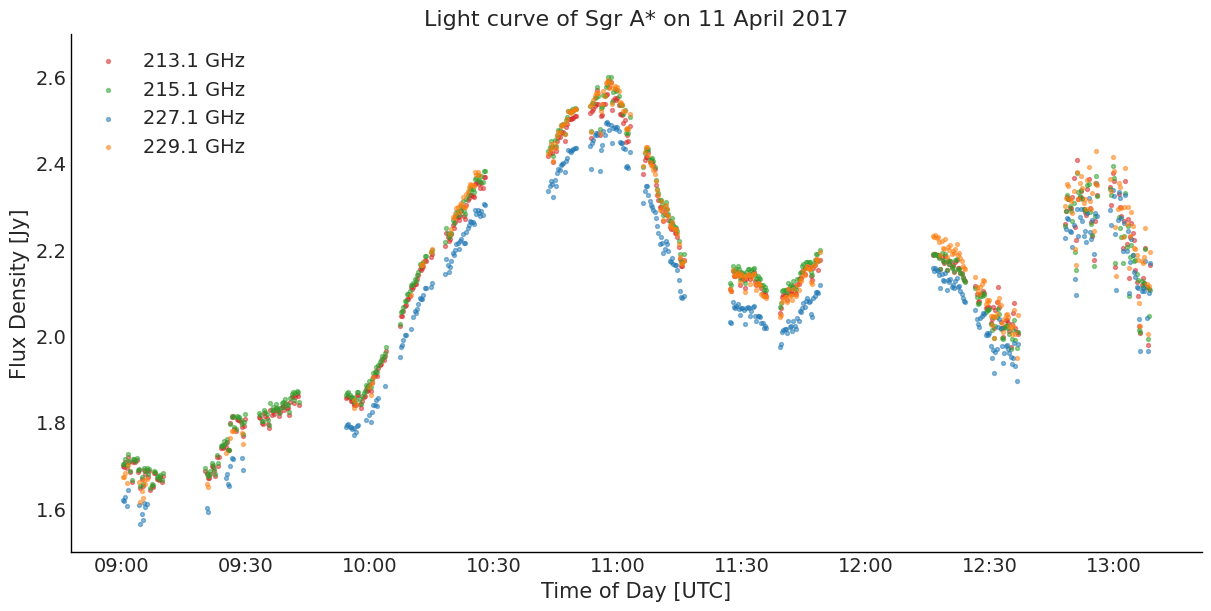
Multi-band Light Curve
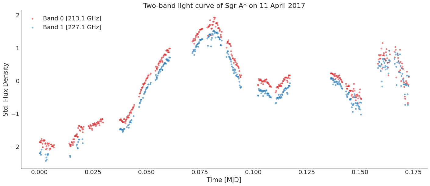
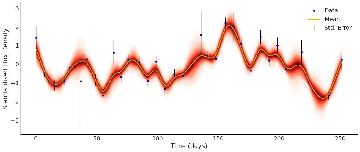
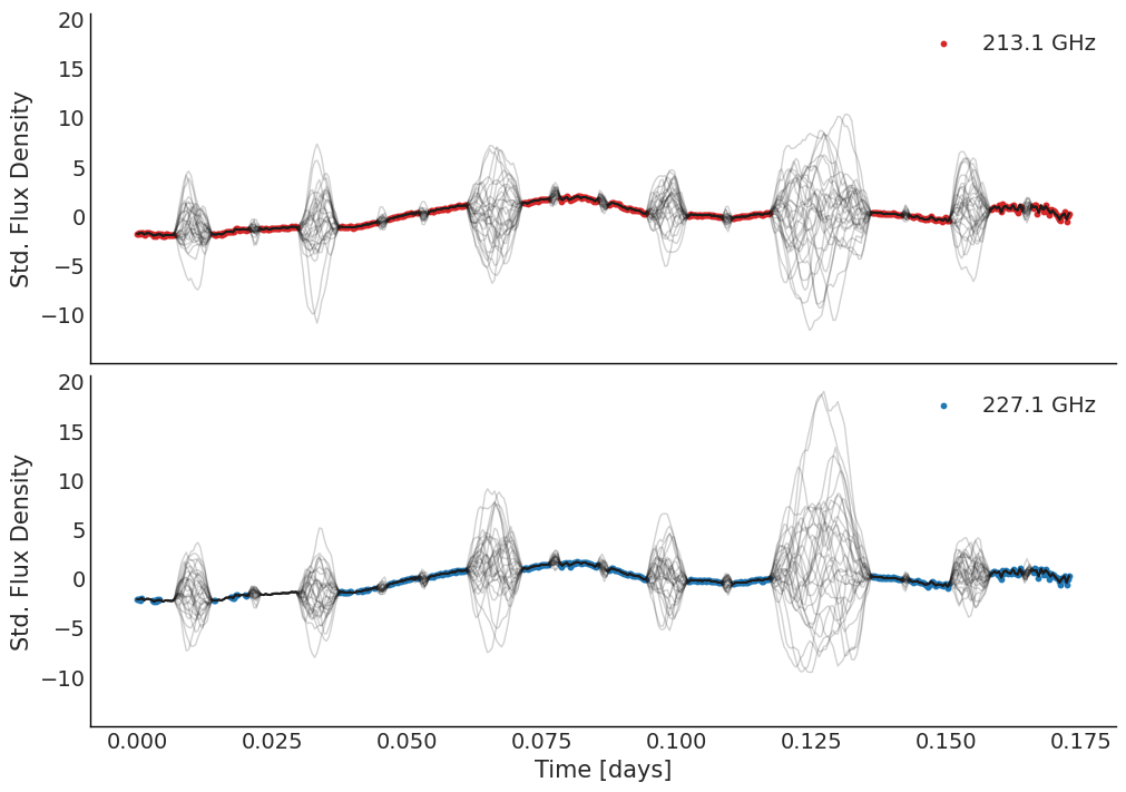
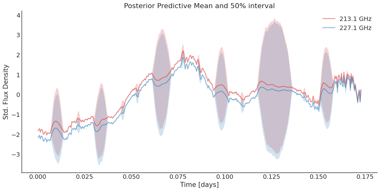
Two-band Light Curve
Gaussian Processes (GPs)
Extend multivariate Gaussian to 'infinite' dimensions.
- Mean function, \(\mu(t)\)
- Covariance or kernel function, \( \kappa(t,t'; \boldsymbol{\theta}) \)
\begin{bmatrix}
Y_1 \\
Y_2 \\
\vdots \\
\end{bmatrix} \sim \mathcal{GP} (\mu(t), \boldsymbol{K})
where \(\mu = \mu(t)\) and \( K_{ij} = \kappa(t_i, t_j; \boldsymbol{\theta}) \), for \( i,j = 1, 2, \dots \)
Rather than specify a fixed covariance matrix with fixed dimensions, compute covariances using the kernel function.
\boldsymbol{K} =
\begin{bmatrix}
K_{11} & \dots & K_{1.} \\
\vdots & \ddots & \vdots \\
K_{.1} & \dots & K_{..}
\end{bmatrix}
Multivariate Normal
Y is a vector of n Gaussian distributed random variables.
\begin{bmatrix}
Y_1 \\
\vdots \\
Y_n
\end{bmatrix} \sim \mathcal{N}_n (\boldsymbol{\mu}, \boldsymbol{\Sigma}_{n \times n})
\boldsymbol{\Sigma}_{n \times n} =
\begin{bmatrix}
\Sigma_{11} & \dots & \Sigma_{1n} \\
\vdots & \ddots & \vdots \\
\Sigma_{n1} & \dots & \Sigma_{nn}
\end{bmatrix}
where \(\boldsymbol\mu = (\mu_1, \dots, \mu_n)\) and \(\boldsymbol{\Sigma}\) is a \(n \times n \) covariance matrix.

\mathbf{\Sigma} =
\begin{bmatrix}
1 & 0 \\
0 & 1
\end{bmatrix}
\mathbf{\Sigma} =
\begin{bmatrix}
1 & 0.8 \\
0.8 & 1
\end{bmatrix}
- Symmetric, positive semi-definite matrix.
- Linear combinations are also valid covariance matrices.
"Single-output" GP
f(\boldsymbol{x}) \sim \mathcal{GP}(\boldsymbol{0}, \kappa(\boldsymbol{x}, \boldsymbol{x}'; \boldsymbol{\theta}))
y(\boldsymbol{x}_i) = f(\boldsymbol{x}_i) + \varepsilon_i
\varepsilon_i \sim \mathcal{N}(0, \sigma^2)
\begin{bmatrix}
y(\boldsymbol{x}_1)\\
\vdots \\
y(\boldsymbol{x}_n)
\end{bmatrix} \sim \mathcal{N}\left(\begin{bmatrix}0\\ \vdots \\ 0 \end{bmatrix},
\begin{bmatrix}
\kappa(\boldsymbol{x}_1, \boldsymbol{x}_1) & \dots & \kappa(\boldsymbol{x}_1, \boldsymbol{x}_n) \\
\vdots & \ddots & \vdots \\
\kappa(\boldsymbol{x}_n, \boldsymbol{x}_1) & \dots & \kappa(\boldsymbol{x}_n, \boldsymbol{x}_n)
\end{bmatrix} + \sigma^2
\begin{bmatrix}
1 & \dots & 0 \\
\vdots & \ddots & \vdots \\
0 & \dots & 1
\end{bmatrix}\right)
\boldsymbol{y} \sim \mathcal{N}(\boldsymbol{0}, \boldsymbol{K} + \sigma^2 \boldsymbol{I})
Multiple Output GP (MOGP)
\begin{bmatrix}
\boldsymbol{y}_1\\
\boldsymbol{y}_2
\end{bmatrix} \sim \mathcal{N}\left(\begin{bmatrix}\boldsymbol{0}\\ \boldsymbol{0} \end{bmatrix},
\begin{bmatrix}
\boldsymbol{K}_1 & \boldsymbol{0} \\
\boldsymbol{0} & \boldsymbol{K}_2
\end{bmatrix} +
\begin{bmatrix}
\sigma^2_1 \boldsymbol{I} & \boldsymbol{0} \\
\boldsymbol{0} & \sigma^2_2 \boldsymbol{I}
\end{bmatrix}\right)
\boldsymbol{y} \sim \mathcal{N}(\boldsymbol{0}, \boldsymbol{K}_{\boldsymbol{f},\boldsymbol{f}} + \boldsymbol{\Sigma})
\(1 \times (n_1 + n_2)\)
\((n_1 + n_2) \times (n_1 + n_2)\)
Cross-covariance
\(\boldsymbol{K}_{\boldsymbol{f},\boldsymbol{f}}\)
f_1(\boldsymbol{x}) \sim \mathcal{GP}(\boldsymbol{0}, \kappa_1(\boldsymbol{x}, \boldsymbol{x}'))
\boldsymbol{y}_1 \sim \mathcal{N}(\boldsymbol{0}, \boldsymbol{K}_1 + \sigma^2_1 \boldsymbol{I})
\mathcal{D}_1 = \{ ( \boldsymbol{x}_{i,1}, y_1(\boldsymbol{x}_{i,1}) ) ; i = 1, \dots, n_1\}
f_2(\boldsymbol{x}) \sim \mathcal{GP}(\boldsymbol{0}, \kappa_2(\boldsymbol{x}, \boldsymbol{x}'))
\boldsymbol{y}_2 \sim \mathcal{N}(\boldsymbol{0}, \boldsymbol{K}_2 + \sigma^2_2 \boldsymbol{I})
\mathcal{D}_2 = \{ ( \boldsymbol{x}_{i,2}, y_2(\boldsymbol{x}_{i,2}) ) ; i = 1, \dots, n_2\}
MOGP Kernels
- Choose a cross-covariance function \( \operatorname{cov}[f_1(\boldsymbol{x}),f_2(\boldsymbol{x}')]\) such that \( \boldsymbol{K}_{\boldsymbol{f},\boldsymbol{f}}\) is a valid covariance matrix, i.e., positive semi-definite.
- Start with "separable" kernels where \(\boldsymbol{K}_{\boldsymbol{f},\boldsymbol{f}}\) is decomposed into submatrices.
\begin{bmatrix}
\boldsymbol{f}_1\\
\boldsymbol{f}_2
\end{bmatrix} \sim \mathcal{N}\left(\begin{bmatrix}\boldsymbol{0}\\ \boldsymbol{0} \end{bmatrix},
\begin{bmatrix}
\boldsymbol{K}_1 & \\
& \boldsymbol{K}_2
\end{bmatrix} +
\begin{bmatrix}
\sigma^2_1 \boldsymbol{I} & \boldsymbol{0} \\
\boldsymbol{0} & \sigma^2_2 \boldsymbol{I}
\end{bmatrix}\right)
\(\boldsymbol{K}_{\boldsymbol{f},\boldsymbol{f}}\)
?
?
Semiparametric Latent Factor Model (SLFM)
Fit each band as a linear combination of two latent GPs,
where \(d = 1,2,3,4\) output bands and \(q = 1,2\) latent processes
\begin{align*}
\begin{bmatrix}
\boldsymbol{f}_1\\
\boldsymbol{f}_2\\
\boldsymbol{f}_3\\
\boldsymbol{f}_4\\
\end{bmatrix} &=
\begin{bmatrix}
a_{1,1} & a_{1,2} \\
a_{2,1} & a_{2,2} \\
a_{3,1} & a_{3,2} \\
a_{4,1} & a_{4,2}
\end{bmatrix} \times
\begin{bmatrix}
u_1(\boldsymbol{x}) \\
u_2(\boldsymbol{x})
\end{bmatrix} =
\begin{bmatrix}
\boldsymbol{a}_1 & \boldsymbol{a}_2
\end{bmatrix} \times
\begin{bmatrix}
u_1(\boldsymbol{x}) \\
u_2(\boldsymbol{x})
\end{bmatrix}
\end{align*}
\boldsymbol{f}(\boldsymbol{x}) = \boldsymbol{a}_1 u_1 (\boldsymbol{x}) + \boldsymbol{a}_1 u_2 (\boldsymbol{x})
\begin{align*}
u_1(\boldsymbol{x}) &\sim \mathcal{GP}(\boldsymbol{0}, \kappa_1(x, x'))\\
u_2(\boldsymbol{x}) &\sim \mathcal{GP}(\boldsymbol{0}, \kappa_2(x, x'))
\end{align*}
f_d(\boldsymbol{x}) = \sum^4_q a_{d,q} u_q(\boldsymbol{x})
Alternatively,
Semiparametric Latent Factor Model (SLFM)
\begin{align*}
\boldsymbol{K}_{\boldsymbol{f},\boldsymbol{f}} &=
\begin{bmatrix}
\mathrm{cov}[f_1(\boldsymbol{x}), f_1(\boldsymbol{x'})] & \dots & \mathrm{cov}[f_1(\boldsymbol{x}), f_4(\boldsymbol{x'})]\\
\vdots & \ddots & \vdots \\
\mathrm{cov}[f_1(\boldsymbol{x'}), f_4(\boldsymbol{x})] & \dots & \mathrm{cov}[f_4(\boldsymbol{x}), f_4(\boldsymbol{x'})]
\end{bmatrix} \\
&= \sum^2_q \boldsymbol{a}_q \boldsymbol{a}_q^\top \otimes \kappa_q(\boldsymbol{x}, \boldsymbol{x}') \\
&= \sum^2_q \boldsymbol{B}_q \otimes \boldsymbol{K}_{f_q, f_q}
\end{align*}
Co-regionalisation Matrices
Kronecker product
Latent Process Model
\begin{align*}
[\boldsymbol{K}_{f_1, f_1}]_{i, j} &= \kappa_1(x, x'; \sigma_{\textrm{M32}}, \ell_{\textrm{M32}})\\
&= \sigma_\textrm{M32}^2 \left(1 + \sqrt{3}\frac{(x - x')^2}{\ell_\textrm{M32}}\right)\exp\left[-\sqrt{3}\frac{(x - x')^2}{\ell_\textrm{M32}}\right]
\end{align*}
\begin{gather*}
\sigma_\textrm{SE}, \sigma_\textrm{M32} \sim \mathcal{N}^+(0,1) \\
\ell_\textrm{SE}, \ell_\textrm{M32} \sim \mathrm{InvGamma}\left(\alpha = 3, \beta = \frac{1}{2} \times \lceil\textrm{range}(t)\rceil\right) \\
\ell_\textrm{SE}, \ell_\textrm{M32} > \textrm{min}(\Delta t) \\
\ell_\textrm{SE} > \ell_\textrm{M32} \\
\end{gather*}
Parameter model
u_1(\boldsymbol{x}) \sim \mathcal{GP}(\boldsymbol{0}, \kappa_1(x, x')) \qquad
u_2(\boldsymbol{x}) \sim \mathcal{GP}(\boldsymbol{0}, \kappa_2(x, x'))
\begin{gather*}
\sigma_{\textrm{M32}}, \sigma_{\textrm{SE}} \sim \mathcal{N}^+(0,1) \\
\ell_{\textrm{M32}}, \ell_{\textrm{SE}} \sim \mathrm{InvGamma}\left(\alpha = 3, \beta = \frac{1}{2} \times \lceil\textrm{range}(t)\rceil\right) \\
\ell_{\textrm{M32}}, \ell_{\textrm{SE}} > \textrm{min}(\Delta t) \\
\ell_{\textrm{SE}} > \ell_{\textrm{M32}} \\
\end{gather*}
[\boldsymbol{K}_{f_2, f_2}]_{i, j} = \kappa_2(x, x'; \sigma_{\textrm{SE}}, \ell_{\textrm{SE}}) = \sigma_{\textrm{SE}}^2 \exp\left\{ -\frac{(x - x')^2}{2\ell_{\textrm{SE}}^2}\right\}
Matern 3/2
Squared Exponential
Interested in the length scale hyperparameters \(\ell_{\textrm{M32}}\) and \(\ell_{\textrm{SE}}\)
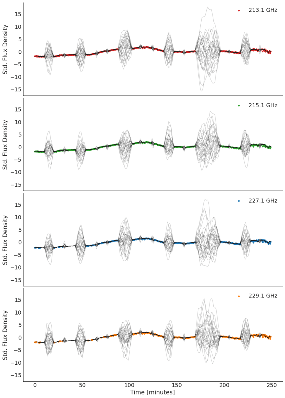
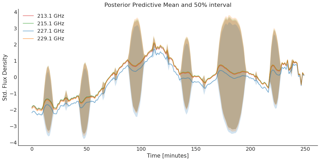
Four-band Light Curve
SLFM Fitting Result
\(\ell_{M32}\) = 7.20 minutes (94% HDI 4.32, 8.64)
\(\ell_{SE}\) = 33.1 minutes (94% HDI 27.4, 38.9)
NB: Fitted curves are perfectly aligned.
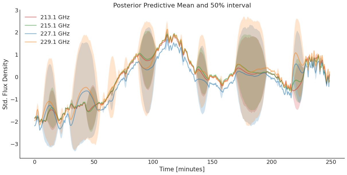
SLFM Result
\(\ell_{M32}\) = 7.23 minutes (94% HDI 5.04, 9.65)
\(\ell_{SE}\) = 25.6 minutes (94% HDI 18.9, 30.2)
NB: Fitted curves are perfectly aligned.
SLFM Fitting Result
\(\ell_{M32}\) = 7.20 minutes (94% HDI 4.32, 8.64)
\(\ell_{SE}\) = 33.1 minutes (94% HDI 27.4, 38.9)
NB: Fitted curves are perfectly aligned.
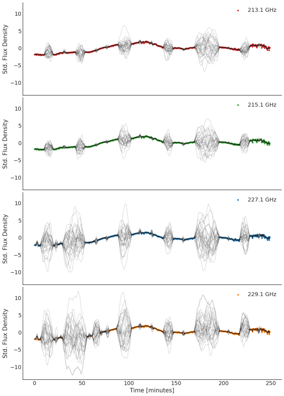
Naive Estimation of Band Delay
- Cross-correlation is a commonly used method to identify the lag between time series.
- But unevenly sampled data complicates this.
- Try resampling the data with a GP model and then compute cross-correlation between posterior predictive samples.
- Separable MOGPs obliterate time-delay information.
4-band
Light Curve
Fit 4 univariate GPs
Cross-correlation on posterior samples
Identify most likely time delay
Four Single-output GPs
\boldsymbol{K}_{\boldsymbol{f},\boldsymbol{f}} = \begin{bmatrix}
\boldsymbol{K}_1 & \boldsymbol{0} & \boldsymbol{0} & \boldsymbol{0} \\
\boldsymbol{0} & \boldsymbol{K}_2 & \boldsymbol{0} & \boldsymbol{0} \\
\boldsymbol{0} & \boldsymbol{0} & \boldsymbol{K}_3 & \boldsymbol{0} \\
\boldsymbol{0} & \boldsymbol{0} & \boldsymbol{0} & \boldsymbol{K}_4
\end{bmatrix}
[\boldsymbol{K}_q]_{i, j} = \kappa_{q_\textrm{M32}}(x_i, x_j; \sigma_{q_\textrm{M32}}, \ell_{q_\textrm{M32}}) + \kappa_{q_\textrm{SE}}(x_i, x_j; \sigma_{q_\textrm{SE}}, \ell_{q_\textrm{SE}})
Cross Correlation
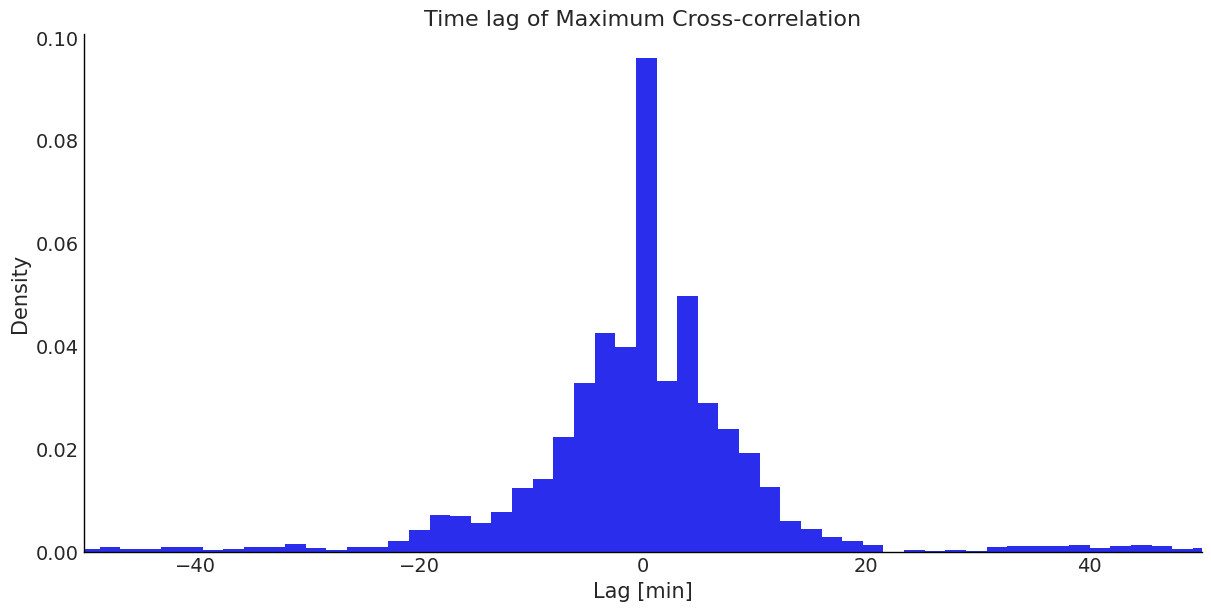
- Results are poor, most lags at zero.
- Model the time-delay term explicitly!
- Considering Spectral Mixture Kernel MOGPs
"Stop using computer simulations as a substitute for thinking"
Quantitude Podcast, Season 4, Episode 7
Summary
- Multi-band light curves of Sgr A* with different sampling rates.
- Tried using MOGP regression to characterise the:
- time scale of variation, and
- time delays between bands.
- Found two characteristic time scales: 7.2 and 33.1 minutes.
- Separable kernels cannot be used to model the cross-band time delays; need to parameterise these explicitly.
- Navigating the literature between astronomy, astrophysics, statistics, and machine learning, has been tricky.
Characterising the Variability of the Black Hole at the Centre of our Galaxy using Multi-Output Gaussian Processes
By Shih Ching Fu
Characterising the Variability of the Black Hole at the Centre of our Galaxy using Multi-Output Gaussian Processes
Multi-Output Gaussian Process (MOGP) regression extends univariate Gaussian Process regression to cases where multiple response variables should be modelled together. For example, these may be response variables that co-vary because they share an underlying origin. This makes MOGP regression perfectly suited for modelling the multi-band data collected by astronomical facilities such as the Atacama Large Millimeter/submillimeter Array (ALMA). In this instance, the multiple outputs correspond to the brightness of emissions from a celestial source as detected at different electromagnetic (EM) frequencies. Here, the celestial source is Sagittarius A* (Sgr A*), the supermassive black hole (SMBH) at the Galactic centre of the Milky Way, and we assume that its changing brightness over time, known as its light curve, is a stochastic process. Using a Bayesian hierarchical model, we demonstrate how MOGPs can be used to infer the relationship between the brightnesses observed at different frequency bands, known as the spectral index. We compare the results of different modelling decisions, such as the choice of cross-covariance structure, and despite light curves being notoriously sparse and unevenly sampled, we obtain a reasonable estimate of the spectral index. Astronomers are interested in the spectral index because it offers clues to the mechanism behind the EM emission.
