


Clayton Shonkwiler PRO
Mathematician and artist
/geotop-a-23
this talk!
Seminar GEOTOP–A, Nov. 17, 2023
Florida State University
National Science Foundation (DMS–2107700)
Simons Foundation (#709150)
The Ohio State University
Johns Hopkins University
Signal: \(v \in \mathbb{C}^d\).
Design: Choose \(f_1, \dots , f_n \in \mathbb{C}^d\) (a frame).
Measurements: \(\langle f_1, v \rangle, \dots , \langle f_n, v \rangle \).
Goal: Reconstruct the signal \(v\) from \(F^* v\)
If \(F = \begin{bmatrix} f_1 & \cdots & f_n\end{bmatrix}\), the measurement vector is \(F^*v\).
If \(f_1,\dots , f_d\in \mathbb{C}^d\) form an orthonormal basis, then
\(v=\sum \langle f_k,v\rangle f_k = FF^* v\).
\(\Leftrightarrow FF^* = \mathrm{Id}_{d \times d}\)
This is fragile! What if a measurement gets lost?
Definition.
\(\{f_1,\dots, f_n\}\subset \mathbb{C}^d\) is a Parseval frame if \(\operatorname{Id}_{d\times d}=FF^*=f_1f_1^*+\dots+f_nf_n^*\).
The rows of \(F\) form an orthonormal set in \(\mathbb{C}^n\), so the space of all length-\(n\) Parseval frames in \(\mathbb{C}^d\) is the Stiefel manifold \(\operatorname{St}_d(\mathbb{C}^n)\).
Lost measurements are still a problem:
\(F=\begin{bmatrix} 1/\sqrt{2} & 1/\sqrt{2} & 0 \\ 0 & 0 & 1 \end{bmatrix}\)
An equal-norm Parseval frame (ENP frame) is a Parseval frame \(f_1,\dots , f_n\) with \(\|f_i\|^2=\|f_j\|^2\) for all \(i\) and \(j\).
Theorem [Casazza–Kovačevic, Goyal–Kovačevic–Kelner, Holmes–Paulsen]
ENP frames are optimal for signal reconstruction in the presence of white noise and erasures.
\(\sum \|f_i\|^2=\operatorname{tr}F^*F=\operatorname{tr}FF^*=\operatorname{tr}\operatorname{Id}_{d \times d} = d\), so each \(\|f_i\|^2=\frac{d}{n}\).
\(\operatorname{spec}(FF^*) = (\lambda_1, \dots , \lambda_d)\)
\((\|f_1\|^2, \dots , \|f_n\|^2)\)
choose based on noise model
detector power
Questions:
A symplectic manifold is a smooth manifold \(M\) together with a closed, non-degenerate 2-form \(\omega \in \Omega^2(M)\).
Example: \((\mathbb{R}^2,dx \wedge dy) = (\mathbb{C},\frac{i}{2}dz \wedge d\bar{z})\)
Non-Example: \((\mathbb{R}^3, dx \wedge dy)\)
For any vector \(v\), \(dx \wedge dy\left(\frac{\partial}{\partial z}, v\right) = 0\), so \(dx \wedge dy\) is degenerate.
Non-Example: \((\mathbb{R}^4, dx_1 \wedge dy_1 + y_1 dx_2 \wedge dy_2)\)
\(d(dx_1 \wedge dy_1 + y_1 dx_2 \wedge dy_2) = dy_1 \wedge dx_2 \wedge dy_2 \neq 0\)
\((S^2,d\theta\wedge dz)\)
\((\mathbb{R}^2,dx \wedge dy) = (\mathbb{C},\frac{i}{2}dz \wedge d\bar{z})\)
\((S^2,\omega)\), where \(\omega_p(u,v) = (u \times v) \cdot p\)
\((\mathbb{R}^2,\omega)\) where \(\omega(u,v) = \langle i u, v \rangle \)
\((\mathbb{C}^n, \frac{i}{2} \sum dz_k \wedge d\overline{z}_k)\)
\((\mathbb{C}^{m \times n}, \omega)\) with \(\omega(X_1,X_2) = -\operatorname{Im} \operatorname{trace}(X_1^* X_2)\).
\((T^* \mathbb{R}^n,\sum dq_i \wedge dp_i)\)
phase space
position
momentum
\(\omega^{\wedge n} = \omega \wedge \dots \wedge \omega\) is a volume form on \(M\), and induces a measure
called Liouville measure on \(M\).
In particular, if \(M\) is compact, this can be normalized to give a probability measure.
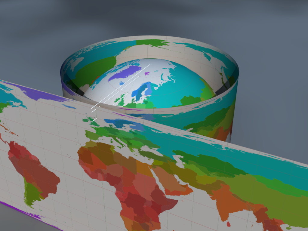
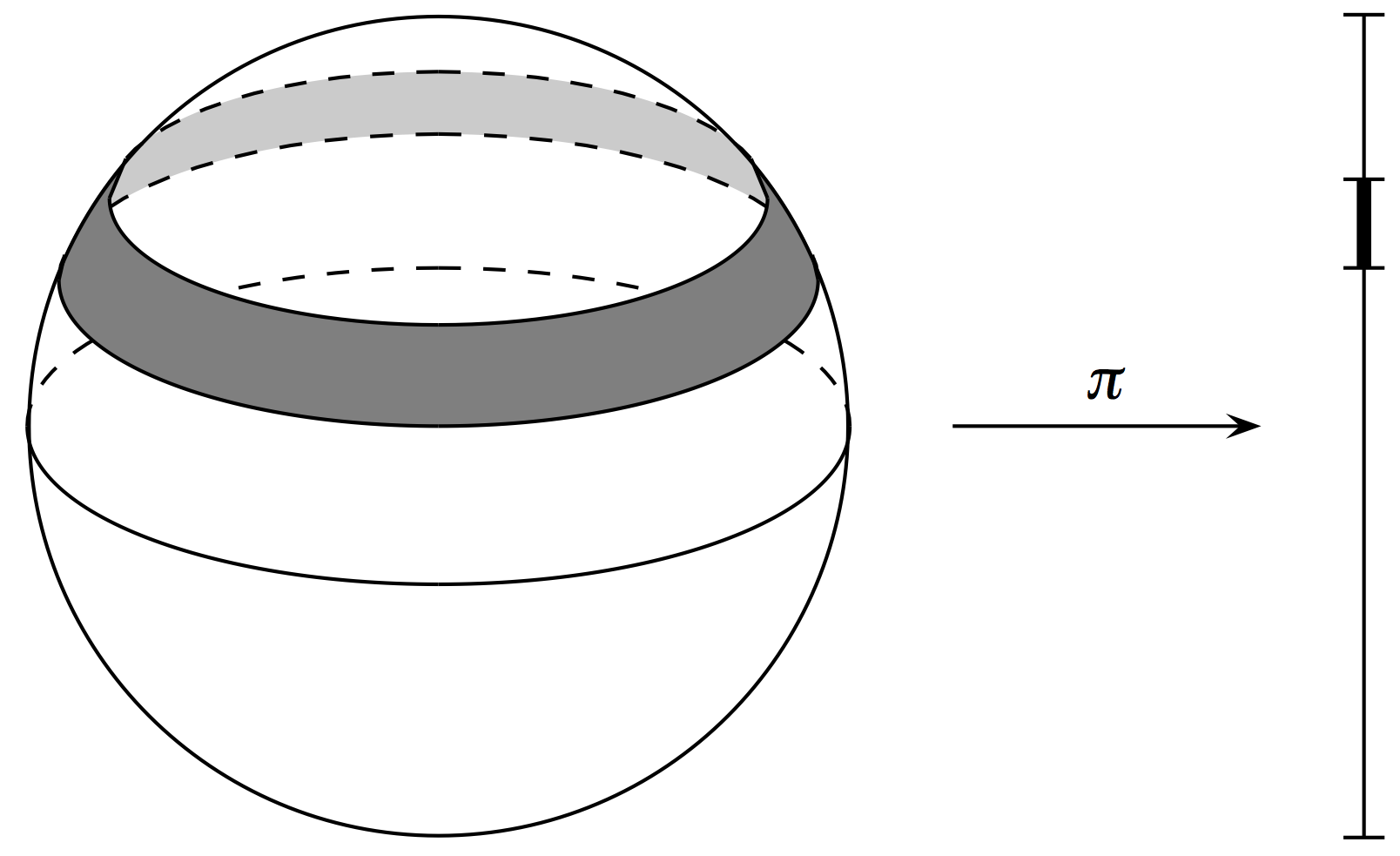
Theorem [Archimedes]
\(\mathrm{d}\theta \wedge \mathrm{d}z\) is the standard area form on the unit sphere \(S^2\).
KoenB [ ] from Wikimedia Commons
“Evolution of a physical system follows the symplectic gradient”
If \(H: M \to \mathbb{R}\) is smooth, then there exists a unique vector field \(X_H\) so that \({dH = \iota_{X_H}\omega}\), i.e.,
(\(X_H\) is called the Hamiltonian vector field for \(H\), or sometimes the symplectic gradient of \(H\))
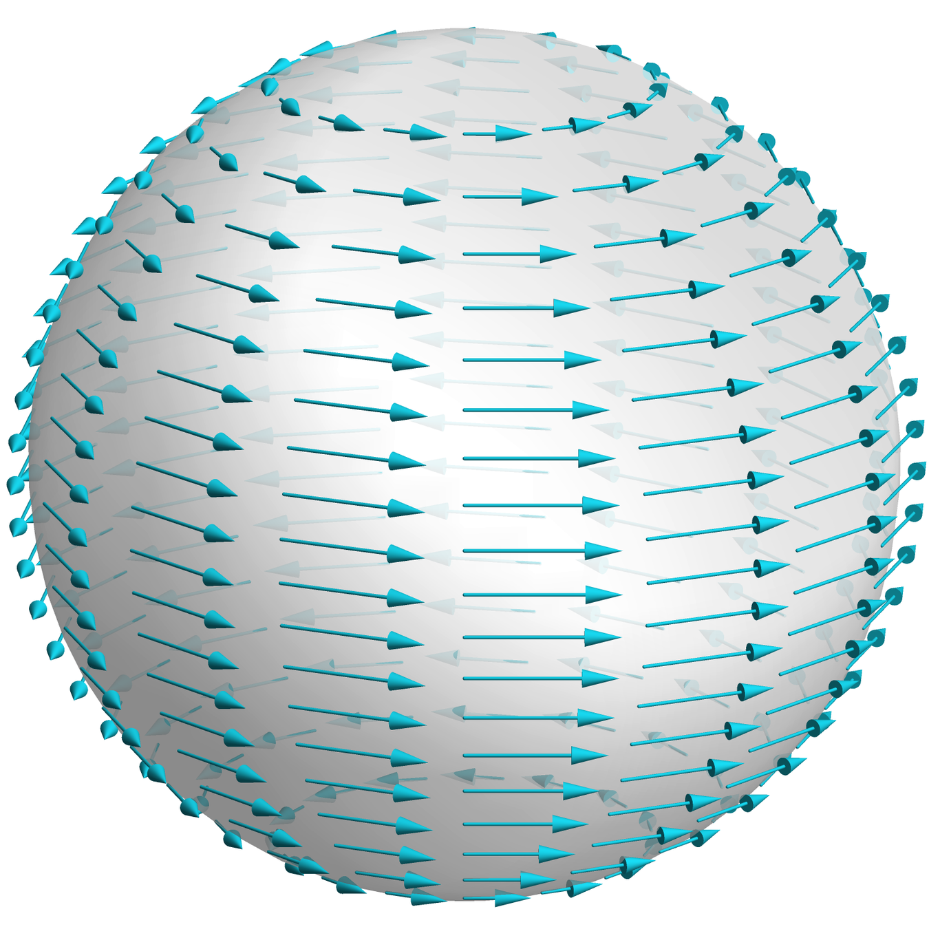
Example. \(H: (S^2, d\theta\wedge dz) \to \mathbb{R}\) given by \(H(\theta,z) = z\).
\(dH = dz = \iota_{\frac{\partial}{\partial \theta}}(d\theta\wedge dz)\), so \(X_H = \frac{\partial}{\partial \theta}\).
\(H\) is constant on orbits of \(X_H\):
\(\mathcal{L}_{X_H}(H) = dH(X_H)=\omega(X_H,X_H) = 0\)
Suppose we have a particle of mass \(m\) with position \(\vec{q} = (q_1,q_2,q_3)\).
Suppose the particle is subject to a potential \(V(\vec{q})\).
Newton’s Second Law: \(-\nabla V(\vec{q}) = m \frac{d^2 \vec{q}}{dt^2}\).
Momenta \(p_i := m \frac{dq_i}{dt}\).
\((\vec{q},\vec{p})\in T^*\mathbb{R}^3 \cong \mathbb{R}^6\); canonical symplectic form \(\omega = dq_1 \wedge dp_1 + dq_2 \wedge dp_2 + dq_3 \wedge dp_3\).
Energy function (or Hamiltonian)
\(H(\vec{q},\vec{p}) := \frac{1}{2m}|\vec{p}|^2 + V(\vec{q})\).
\(dH = \sum\left(\frac{\partial H}{\partial p_i} dp_i + \frac{\partial H}{\partial q_i}dq_i\right)\),
\((\vec{q}(t),\vec{p}(t))\) is an integral curve for \(X_H\) if and only if
\(\frac{dq_i}{dt} = \frac{\partial H}{\partial p_i} = \frac{1}{m} p_i\)
\(\frac{dp_i}{dt} = -\frac{\partial H}{\partial q_i} = -\frac{\partial V}{\partial q_i}.\)
This is Newton’s Second Law written as a first-order system!
\(X_H = \sum\left(\frac{\partial H}{\partial p_i} \frac{\partial}{\partial q_i} - \frac{\partial H}{\partial q_i} \frac{\partial}{\partial p_i}\right)\).
“Every continuous symmetry has a corresponding conserved quantity”
A circle action on \((M,\omega)\) determines a vector field \(X\) by
\(S^1=U(1)\) acts on \((S^2,d\theta \wedge dz)\) by
So \(X = \frac{\partial}{\partial \theta}\).
Definition. A circle action on \((M,\omega)\) is Hamiltonian if there exists a map
so that \(d\mu = \iota_{X}\omega = \omega(X,\cdot)\), where \(X\) is the vector field generated by the circle action. In other words, \(X = X_\mu\).
\(X = \frac{\partial}{\partial \theta}\)
\(\mu(\theta,z) = z\)
\(\iota_X\omega = \iota_{\frac{\partial}{\partial \theta}} d\theta \wedge dz = (d\theta \wedge dz)\left(\frac{\partial}{\partial \theta},\cdot \right) = dz \)
Theorem [Atiyah and Guillemin–Sternberg]
If \((M,\omega)\) is symplectic and \(\mathbb{T}=(S^1)^k\) acts in a Hamiltonian fashion, the conserved quantities are recorded by \(\mu:M \to \mathbb{R}^k\) with:
Theorem [Duistermaat–Heckman]
If \(\dim(M)=2n\) and \(\dim(\mathbb{T})=k\), then the pushforward measure on the moment polytope \(\mu(M)\) is absolutely continuous w.r.t. Lebesgue measure, with continuous, piecewise-polynomial density of degree \(\leq n-k\).
In particular, if \(n=k\), then the pushforward measure is a constant multiple of Lebesgue measure.
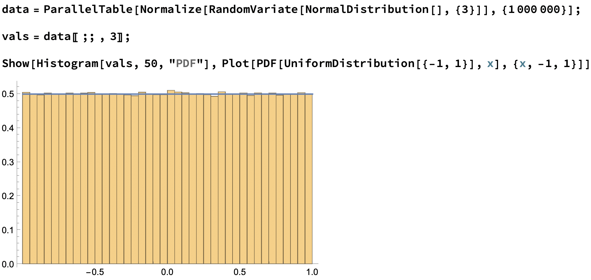
Theorem (Archimedes)
Let \(\mu: S^2 \to \mathbb{R}\) be given by \(\mu(x,y,z) = z\). Pushing forward the uniform measure on \(S^2\) to the image \([-1,1]\) gives (\(2\pi\) times) Lebesgue measure.
Some nice group actions on \(\mathbb{C}^{d \times n}\):
Parseval frames
\(\mu_{U(d)}^{-1}(I_{d\times d})\)
equal-norm frames
\(\mu_{U(1)^N}^{-1}\left(-r,\dots , -r\right)\)
ENPs: \(\mu_{U(d)}^{-1}(I_{d \times d}) \cap \mu_{U(1)^n}^{-1}\left(-\frac{d}{n}, \dots , -\frac{d}{n}\right)\)
Theorem [with Needham]
There is a continuous interpolation between any two frames \(f_1, \dots , f_n\) and \(g_1, \dots , g_n\) with \(\operatorname{spec}(FF^*) = \operatorname{spec}(GG^*)\) and \(\|f_i\| = \|g_i\|\) preserving these conditions.
For compressed sensing, it is desirable to require every minor of the \(d \times n\) matrix \(F\) to be invertible. Such an \(F\) is said to have full spark.
Theorem [with Needham]
Fix the spectrum of \(FF^\ast\) and fix \(\|f_1\|,\dots,\|f_n\|\). There are three possibilities:
Definition [Benedetto–Fickus, Casazza–Fickus]
The frame potential is
\(\operatorname{FP}(f_1,\ldots,f_n) = \|FF^\ast\|_{\operatorname{Fr}}^2\)
Proposition [cf. Welch]
When they exist, the ENP frames are exactly the global minima of \(\operatorname{FP}\).
Theorem [Benedetto–Fickus]
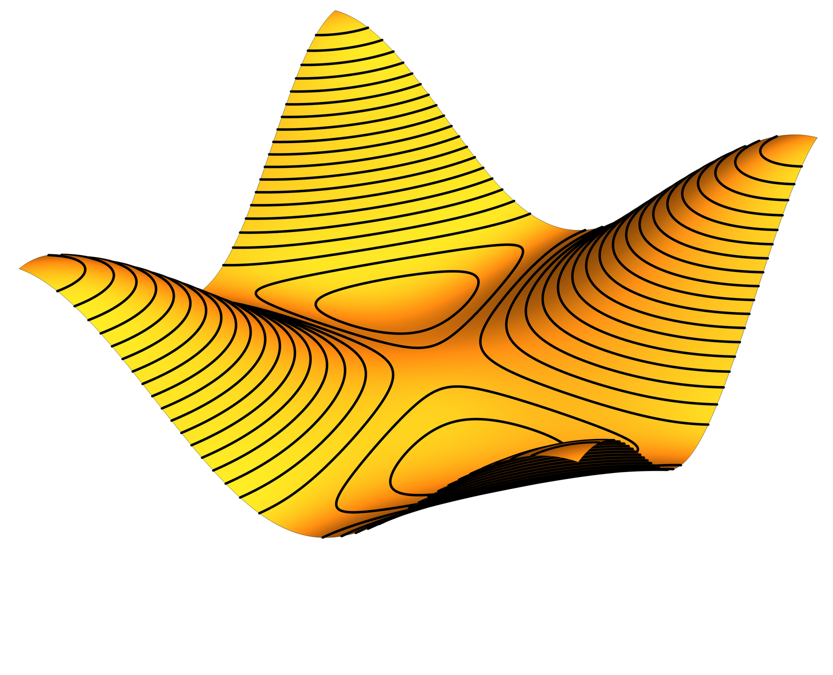
As a function on equal-norm frames with fixed \(d\) and \(n\), \(\operatorname{FP}\) has no spurious local minima.
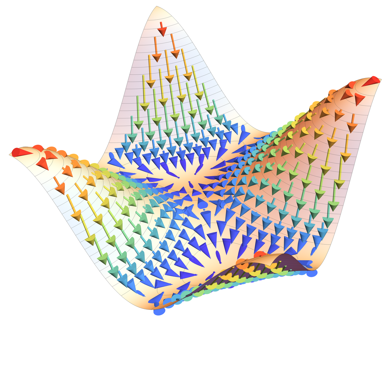
Theorem [with Mixon, Needham, and Villar]
Consider the initial value problem
\(\Gamma(F_0,0) = F_0, \qquad \frac{d}{dt}\Gamma(F_0,t) = -\operatorname{grad}\operatorname{FP}(\Gamma(F_0,t))\).
If \(F_0\) has full spark, then \(\lim_{t \to \infty} \Gamma(F_0,t)\) is an ENP frame.
Theorem [with Needham]
Same for fusion frames.
\(F \mapsto FF^*\) is the momentum map of the diagonal \(SU(d)\) action on \(\prod_{i=1}^n \mathbb{CP}^{d-1}\).
\(\Longrightarrow\) \(\operatorname{FP}(F) = \|FF^*\|_{\operatorname{Fr}}^2\) is the squared norm of a momentum map.
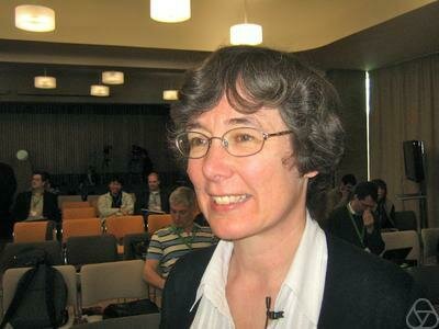
Frances Kirwan
Gert-Martin Greuel [CC BY-SA 2.0 DE], from Oberwolfach Photo Collection
Image by rawpixel.com on Freepik
Theorem [Kirwan]
Reductive algebraic group action on Kähler manifold \(\Longrightarrow\) semistable points flow to global minima.
This kind of function is really nice!
The GIT quotient consists of group orbits which can be distinguished by \(G\)-invariant (homogeneous) polynomials.
\(\mathbb{C}^* \curvearrowright \mathbb{CP}^2\)
\(t \cdot [z_0:z_1:z_2] = [z_0: tz_1:\frac{1}{t}z_2]\)
Roughly: identify orbits whose closures intersect, throw away orbits on which all \(G\)-invariant polynomials vanish.
\( \mathbb{CP}^2/\!/\,\mathbb{C}^* \cong\mathbb{CP}^1\)
An ENP frame \(F\) is equiangular if there exists \(\alpha\) so that \(|\langle f_i , f_j \rangle| = \alpha\) for all \(i \neq j\). Equiangular ENP frames are usually called equiangular tight frames (ETFs).
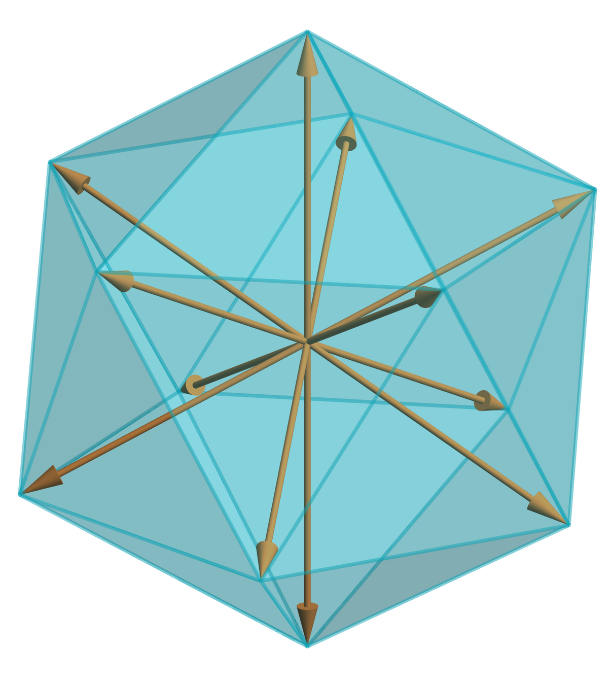
If \(F \in \mathbb{C}^{d \times n}\) is an ETF, then \((f_1f_1^* - \frac{1}{n}\operatorname{Id}_{d \times d}, \dots , f_nf_n^* - \frac{1}{n}\operatorname{Id}_{d \times d})\) are the vertices of a regular \((n-1)\)-simplex in \(\mathscr{H}_0(d) \simeq \mathfrak{su}(d)^\ast\). In particular, this implies \(n \leq d^2\).
(Weak) Zauner Conjecture
For all positive integers \(d\), there exists an ETF \(F \in \mathbb{C}^{d \times d^2}\).
Such ETFs are called maximal ETFs in the math literature, and Symmetric, Informationally-Complete, Positive Operator-Valued Measures (SIC-POVMs) in quantum information theory.
Symplectic geometry and connectivity of spaces of frames
Tom Needham and Clayton Shonkwiler
Advances in Computational Mathematics 47 (2021), no. 1, 5. arXiv:1804.05899
Toric symplectic geometry and full spark frames
Tom Needham and Clayton Shonkwiler
Applied and Computational Harmonic Analysis 61 (2022), 254–287. arXiv:2110.11295
Three proofs of the Benedetto–Fickus theorem
Dustin Mixon, Tom Needham, Clayton Shonkwiler, and Soledad Villar
Sampling, Approximation, and Signal Analysis (Harmonic Analysis in the Spirit of J. Rowland Higgins), Stephen D. Casey, M. Maurice Dodson, Paulo J. S. G. Ferreira and Ahmed Zayed, eds., to appear. arXiv:2112.02916
Fusion frame homotopy and tightening fusion frames by gradient descent
Tom Needham and Clayton Shonkwiler
Journal of Fourier Analysis and Applications 29 (2023), no. 4, 51. arXiv:2208.11045
By Clayton Shonkwiler


