Interpreting systems as solving POMDPs: a step towards a formal understanding of agency
Martin Biehl (Cross Labs)
Nathaniel Virgo (Earth-Life Science Institute)


Made possible via funding by:
Overview
- Background
- Main question
- Moore machine definition
- Informal answer
- Moore machine interpretation via POMDP
- Relation to FEP
- Summary
Overview
- Background on the problem
- Agent definition
- Idea (agent is system-interpretation pair)
- Definition of Moore machines and POMDPs
- Narrative / argumentation
- POMDP solution
- "Belief Moore machine" for solving a POMDP
- Moore machines with interpretation as solving a POMDP
agent!
Background

agents?
What is the difference?


non-agents?

Background
Physics:
- laws of physics are the same everywhere
- no matter whether there is a rock or a human / animal / agent
- no difference?
Background
Daniel Dennett:
- can take various stances towards any object
- stance with better prediction of the object behavior "wins"
Two stances (ignore design stance):
- physical stance: use physical constituents of object and laws of physics
-
intentional stance: assume object
- has beliefs
- has a goal
- acts rationally (=optimally) to achieve goal under its beliefs
Background
Our approach:
- does not apply to actual objects (rocks / animals)
- only applies to well defined/abstract systems (Moore machines)
- does not compare prediction performance of stances
- instead checks whether interpretation in terms of beliefs and goal is consistent with system dynamics
Main question
Given stochastic Moore machine (without any environment):
Question: When is it justified to call it an agent?
Agent definition
Given stochastic Moore machine (without any environment):
Ask: Is it an agent?
We propose: Justified to call it "agent" if together with
-
consistent interpretation in terms of
- beliefs
- goal
- optimal actions to achieve goal according to belief
Agent definition
Given stochastic Moore machine (without any environment):
Question: When is it justified to call it an agent?
We propose answer:
- if find consistent interpretation as a solution to a partially observable Markov decision process (POMDP)
Because this provides well defined notions of
- beliefs
- a goal
- rational/optimal actions
Agent definition
stochastic machine:
- internal state space \(\mathcal{M}\)
- input space \(\mathcal{I}\)
- machine kernel \(\mu:\mathcal{I}\times \mathcal{M}\to P\mathcal{M}\)
write:
- \(\mu(m'|i,m)\) probability of next state \(m'\) given input \(i\) and state \(m\)
- \(\omega(m)\) output in state \(m\)
Agent definition idea
Agent:
- system with
- beliefs
- goal
- actions to achieve the goal.
Agent definition idea
Agent:
- system with interpretation in terms of
- beliefs
- goal
- actions to achieve the goal.
Agent definition idea
Agent:
- system and
-
interpretation in terms of
- beliefs
- goal
- actions to achieve the goal.
Agent definition idea
Agent:
- system and
-
interpretation in terms of
- beliefs
- goal
- actions to achieve the goal.
So agent is a pair of system and interpretation.
Dennett: any interpretation is fine, predictive performance matters.
We: only consistent interpretations are fine
Agent definition idea
Possibly many interesting pairs of
- kinds of systems
- kinds of interpretation
Here choose:
- kind of system: (stochastic) Moore machine
- kind of interpretation: via partially observable Markov decision process (POMDP)
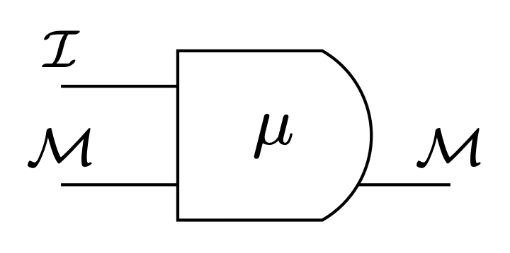
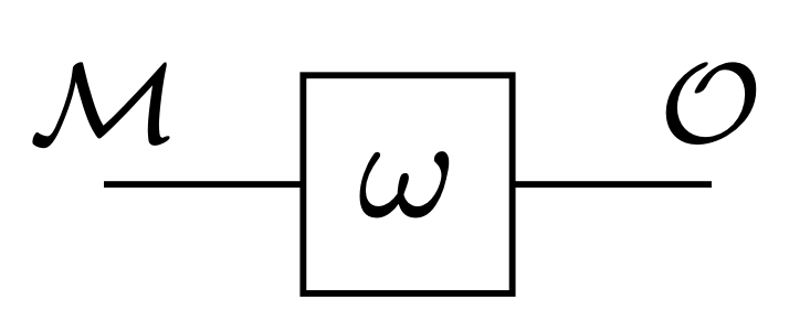
Moore machine definition
stochastic Moore machine:
- internal state space \(\mathcal{M}\)
- input space \(\mathcal{I}\)
- output space \(\mathcal O\)
- machine kernel \(\mu:\mathcal{I}\times \mathcal{M}\to P\mathcal{M}\)
- output function \(\omega: \mathcal M \to \mathcal O\)
notation:
- \(\mu(m'|i,m)\) probability of next state \(m'\) given input \(i\) and state \(m\)
- \(\omega(m)\) output in state \(m\)
Informal answer
Given stochastic Moore machine (without any environment):
Question: When is it justified to call it an agent?
Proposal: Justified to call it "agent" if find
-
consistent interpretation in terms of
- beliefs
- goal
- optimal/rational actions to achieve goal according to belief
Moore machine interpretation via POMDP
Formal answer:
-
consistent interpretation as a solution to a POMDP
-
this consists of
-
a POMDP and
-
its solution (optimal policy on beliefs)
-
interpretation function
-
-
satisfying
-
a consistency equation (Bayesian updating)
-
optimal action equation
-
-
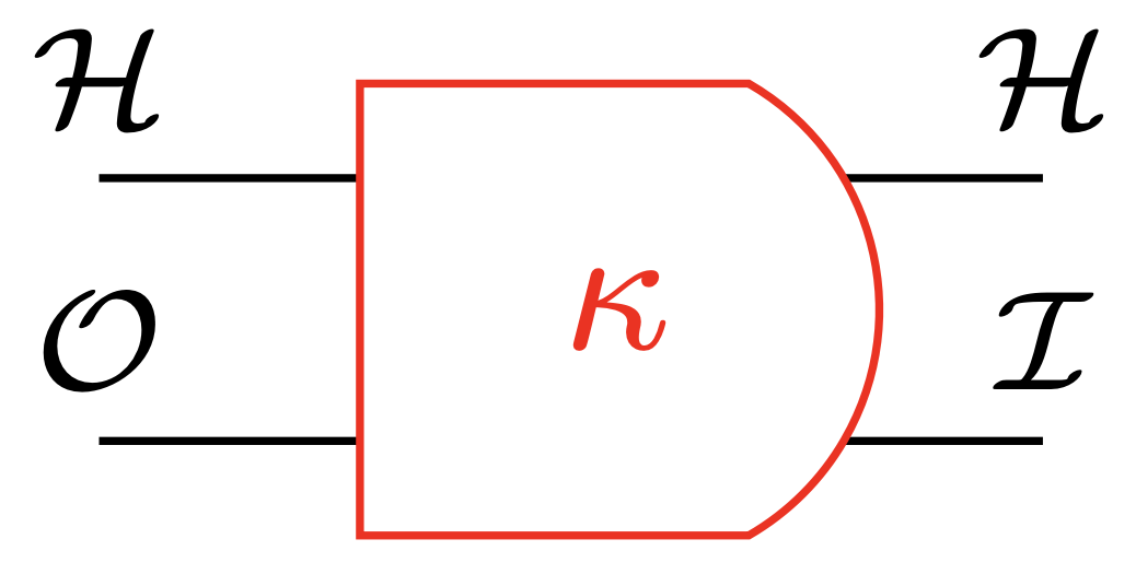
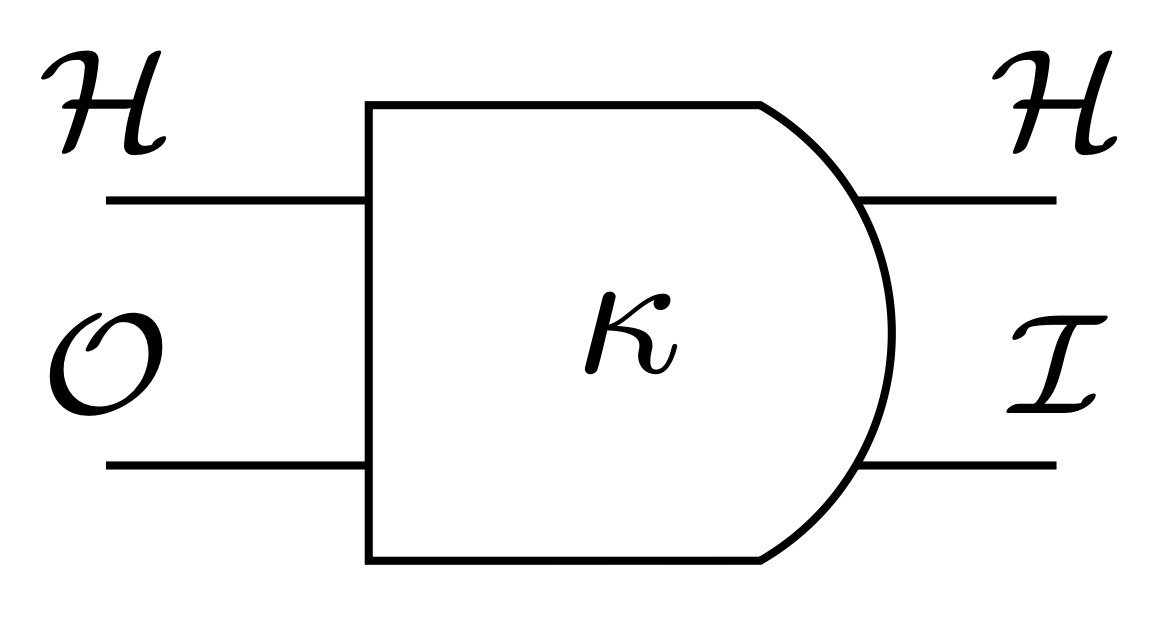
Partially observable Markov decision process (POMDP) consists of:
- hidden state space \(\mathcal{H}\)
- action space := output space \(\mathcal O\)
- sensor space := input space \(\mathcal I\)
- transition kernel \(\kappa:\mathcal{H}\times \mathcal{O}\to P(\mathcal{H}\times\mathcal I)\)
- reward function \(r: \mathcal H \times \mathcal A \to \mathbb R\)
- goal: maximize expected discounted cumulative reward
notation:
- \(\kappa(h',i|h,o)\) probability of next hidden state \(h'\) and input \(i\) given hidden state \(h\) and output \(o\)
Moore machine interpretation via POMDP
Partially observable Markov decision process (POMDP)
- hidden state space \(\mathcal{H}\)
- action space = output space \(\mathcal O\)
- sensor space = input space \(\mathcal I\)
- transition kernel \(\kappa:\mathcal{H}\times \mathcal{O}\to P(\mathcal{H}\times\mathcal I)\)
- reward function \(r: \mathcal H \times \mathcal A \to \mathbb R\)
Solution consists of:
- belief distribution \(b(h) \in P\mathcal H\) over hidden state
- updated according to Bayes rule
Moore machine interpretation via POMDP

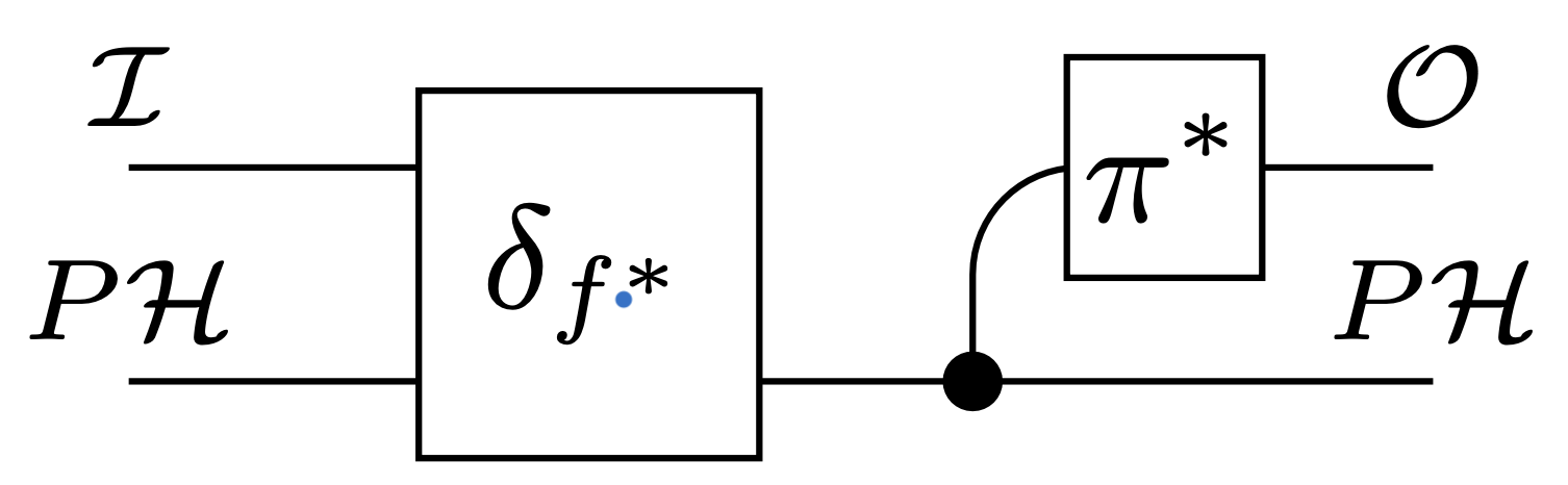
Standard solution of POMDP (well known) induces a Moore machine:
- states are beliefs (=probability distributions) \(b \in P \mathcal H\) over hidden states
- machine kernel \(\delta_{f^*}: \mathcal I \times P \mathcal H \to P\mathcal H\) update beliefs according to Bayes rule
- outputs are optimal policy:
- function \(\pi^*:P\mathcal H \to \mathcal O\) from beliefs over hidden states to actions/outputs
Moore machine interpretation via POMDP
Solution of POMDP (well known):
- introduce beliefs (=probability distributions) over hidden states
- require belief updated according to Bayes rule in response to action (belief MDP)
- then optimal policy is function of beliefs:
- map \(\pi^*:P\mathcal H \to \mathcal O\) from beliefs over hidden states to actions/outputs
Moore machine interpretation via POMDP
POMDP solution
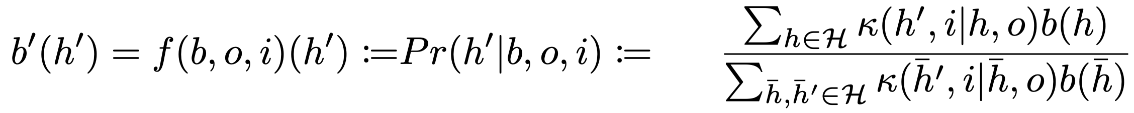
Given a POMDP with hidden state space \(\mathcal H\)
- introduce probability (belief) \(b(h)\) that hidden state is \(h \in \mathcal H\)
- update beliefs according to Bayes rule
- take action / produce output \(o \in \mathcal O\)
- observe sensor value / input \(i \in \mathcal I\)
- then using transition kernel \(\kappa(h',i|h,o)\) Bayes rule specifies how to update the belief distribution to \(b'(h')\):
Standard solution of POMDP (well known) induces a Moore machine:
- states are beliefs (=probability distributions) \(b \in P \mathcal H\) over hidden states
- machine kernel \(\delta_{f^*}: \mathcal I \times P \mathcal H \to P\mathcal H\) update beliefs according to Bayes rule
- outputs are optimal policy:
- function \(\pi^*:P\mathcal H \to \mathcal O\) from beliefs over hidden states to actions/outputs
Moore machine interpretation via POMDP
This machine has beliefs, a goal, and acts optimally \(\Rightarrow\) can call it an agent!
Standard solution of POMDP (well known) induces a Moore machine:
- states are beliefs (=probability distributions) \(b \in P \mathcal H\) over hidden states
- machine kernel \(\delta_{f^*}: \mathcal I \times P \mathcal H \to P\mathcal H\) update beliefs according to Bayes rule
- outputs are optimal policy:
- function \(\pi^*:P\mathcal H \to \mathcal O\) from beliefs over hidden states to actions/outputs
Moore machine interpretation via POMDP
But most machines don't have states that are probability distributions \(\Rightarrow\) can they be agents too?
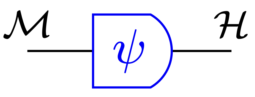
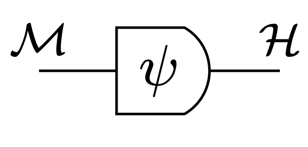
Interpretation function:
- \(\psi:\mathcal M \to P\mathcal H\)
- specifies belief \(\psi(m)\) for each internal state \(m\) of Moore machine
- also write \(\psi(h|m)\) for probability of hidden state \(h \in \mathcal H\) specified for machine state \(m \in \mathcal M\)
Moore machine interpretation via POMDP
Interpretation function:
Moore machine interpretation via POMDP
belief \(\psi(h|m)\) before update
belief \((\psi\circ \mu)(h|i,m)\) after update
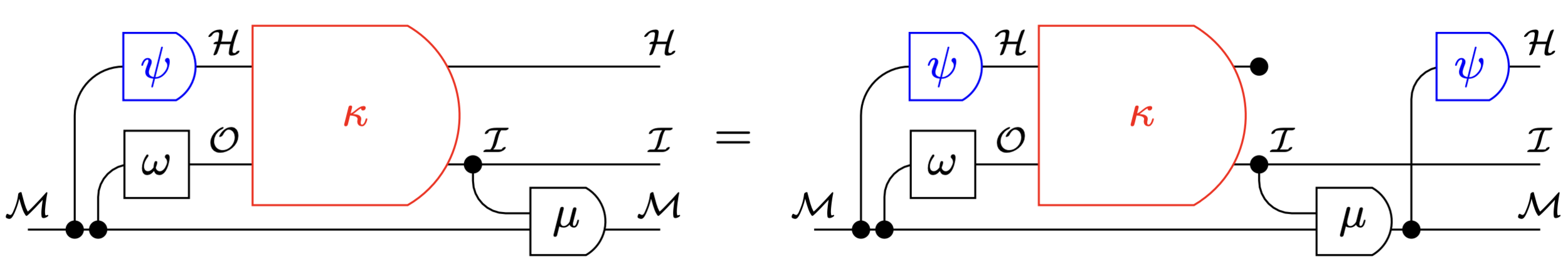
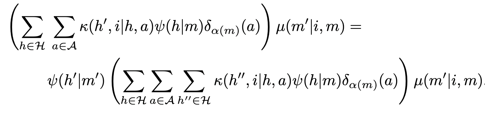
Consistency equation:
- ensures that Bayes rule holds for specified beliefs (not internal states)
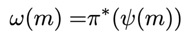
Optimal action equation:
- ensures that output equal to optimal action for specified belief \(\psi(m)\):
Moore machine interpretation via POMDP
Consistency equation:
- ensures that Bayes rule holds for specified beliefs (not internal states)
Optimal action equation:
- ensures that output equal to optimal action for specified belief \(\psi(m)\):
Moore machine interpretation via POMDP
Consistency equation:
- ensures that Bayes rule holds for specified beliefs (not internal states)
Optimal action equation:
- ensures that output function \(\omega\) maps internal states \(m\) to optimal action for specified belief \(\psi(m)\):
Moore machine interpretation via POMDP
Consistency equation:
- with
-
get (deterministic moore machine
- and can get (if not divide by zero)
Moore machine interpretation via POMDP

Can show:
- if Moore machine and interpretation map obey these equations:
- then Moore machine also maximizes expected reward
Reason:
- it updates beliefs specified by \(\psi\) in same way as standard solution
- for each specified belief \(\psi(m)\) it outputs the same action as the standard solution
Moore machine interpretation via POMDP
So interpretation of Moore machine as solution to POMDP has:
- beliefs associated to internal states via interpretation map \(\psi\)
- goal of expected reward maximization
- outputs equal to optimal actions for achieving goal
Justified to call a Moore machine with such an interpretation an agent!
Moore machine interpretation via POMDP
Consistency equation:
- own outputs are taken into account to get posterior
- kind of "active filtering" equation
Optimal action equation:
- machine states determine Bayesian beliefs via interpretation map
- Bayesian beliefs have
Note
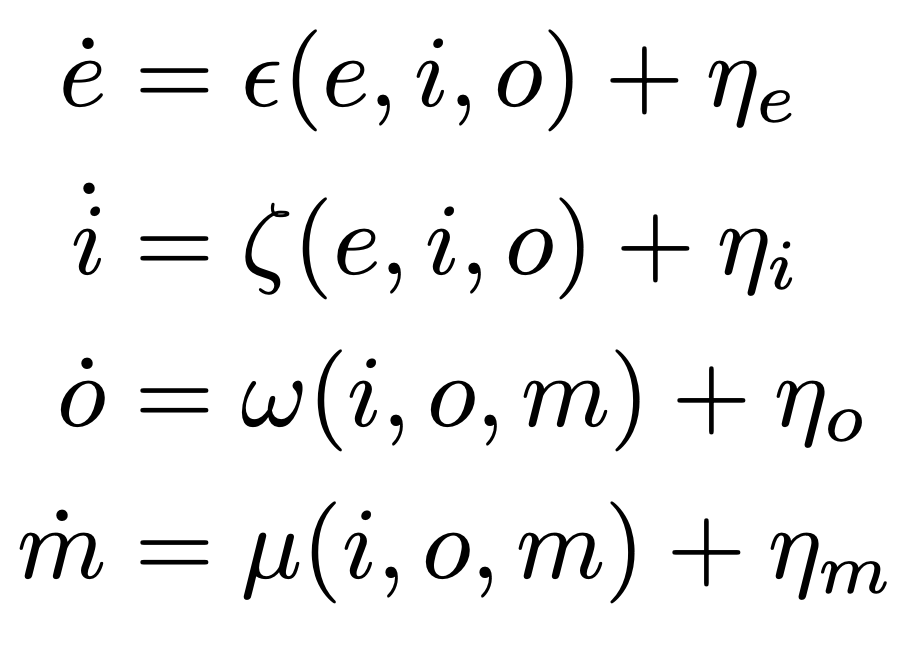
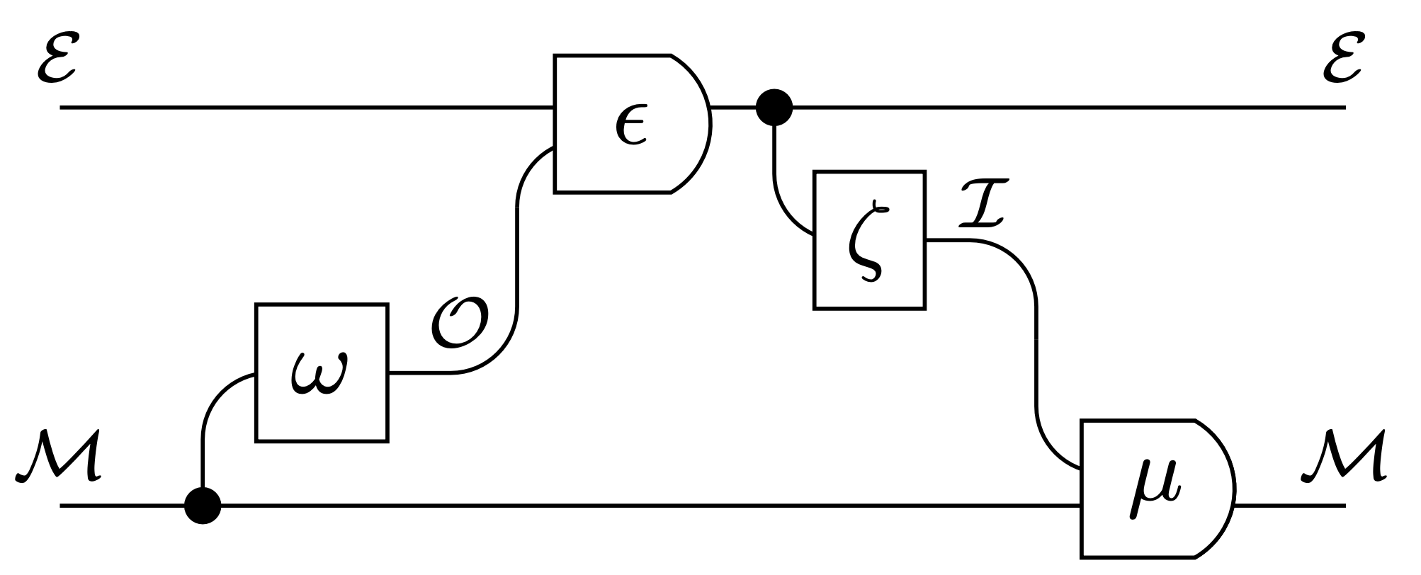
Moore machine analogous to dynamics of autonomous states in FEP:
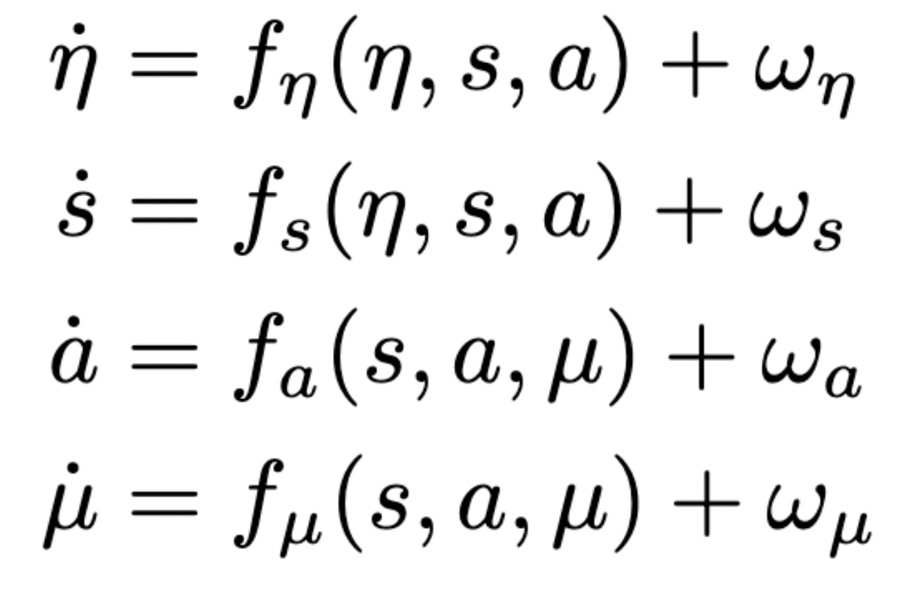
Relation to FEP
Agent definition
Moore machine here plays similar role to dynamics of autonomous states:
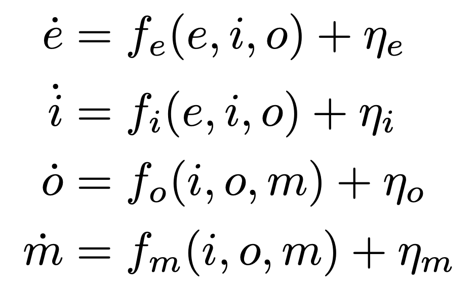
Moore machine here plays similar role to dynamics of autonomous states:
Motivation
Motivation
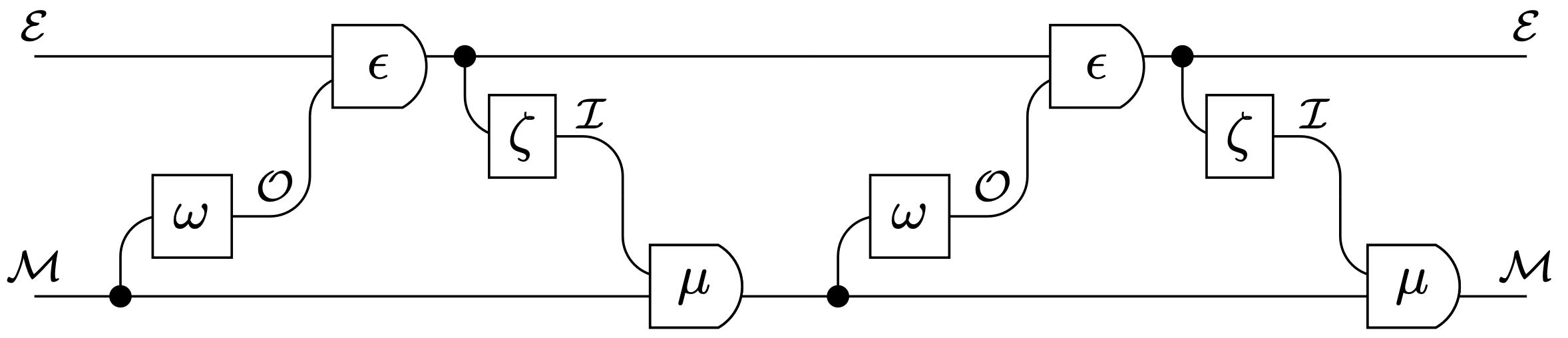
Why are Moore machines interesting?
-
if we have two can combine them:
-
and chain them to get processes:
Moore machine interpretation
So what is a
-
consistent interpretation in terms of
- beliefs
- goal
- optimal actions to achieve goal according to belief
For a Moore machine?
But:
- no assumption of environment
- no ergodicity assumptions
- only need Moore machine to decide about agency!
Relation to FEP
- Showed a way to justify that stochastic Moore machine is an agent
- used:
- standard solutions to POMDPs are basically agents with beliefs, goals, and rationality
- interpretation function extends this to machines whose state spaces aren't probability distributions directly
- Maybe similar approach for other systems exists?
- https://arxiv.org/pdf/2209.01619.pdf
Summary
End
- Agent is consistent pair of system and interpretation
- if we choose
- Moore machines as systems
- interpretation as solution to POMDP
- we gave formal equations to check consistency
- https://arxiv.org/pdf/2209.01619.pdf
Summary
One possible answer:
-
consistent interpretation as a solution to a POMDP
-
this consists of
-
a POMDP i.e.:
- hidden state space \(\mathcal{H}\)
- transition kernel \(\kappa:\mathcal{H}\times \mathcal{O}\to P(\mathcal{H}\times\mathcal I)\)
- reward function \(r: \mathcal H \times \mathcal A \to \mathbb R\)
-
interpretation function \(\psi: \mathcal M \to P\mathcal H\)
-
-
satisfying
-
a consistency equation
-
optimal action equation
-
-
Moore machine interpretation via POMDP
consistency equation
optimal action equation
Moore machine interpretation via POMDP
Moore machine
POMDP transition kernel
interpretation map
consistency equation
optimal action equation
Moore machine interpretation via POMDP
Agent definition
One possible answer:
-
consistent interpretation as a solution to a POMDP
-
this consists of
-
a POMDP
-
interpretation function \(\psi: \mathcal M \to P\mathcal H\)
-
-
satisfying
-
a consistency equation
-
optimal action equation
-
-
Agent definition
One possible answer:
-
consistent interpretation as a solution to a POMDP
-
this consists of
-
a POMDP
-
interpretation function \(\psi: \mathcal M \to P\mathcal H\)
-
-
satisfying
-
a consistency equation
-
optimal action equation
-
-
Agent definition
Lucky observation:
- exist Moore machines that incontrovertibly have such interpretation:
- they solve to partially observable Markov decision processes (POMDPs)
- should count as agents
Then:
- extend set of those Moore machines
Agent definition
Argumentation:
- POMDPs have optimal solutions where
- assume belief (distribution) over hidden state
- update belief via Bayes' rule
- optimal action is function of this belief
- if we consider
- beliefs as internal states
- Bayes rule as machine kernel
- optimal action as output for given belief/internal state
- we get a (deterministic) Moore machine and a justified to say it
- has beliefs
- has a goal (rewards of the POMDP)
- acts rationally according to belief to achieve goal
is an agent!
Agent definition
Argumentation:
- but can extend this:
- internal state space need not be space of belief
- only needs to specify/determine beliefs
- internal state space need not be space of belief
- thus:
- weaker condition on (stochastic) Moore machines exists that guarantees:
- beliefs are specified by internal state
- Bayes rule holds for specified beliefs not internal states directly
- outputs are optimal actions for specified beliefs for given POMDP
- weaker condition on (stochastic) Moore machines exists that guarantees:
also an agent!
POMDP solution
Given a POMDP with hidden state space \(\mathcal H\)
- introduce "belief distribution" \(b:\mathcal H \to [0,1]\) over \(\mathcal H\)
- write \(b(h)\) for probability/confidence that hidden state is \(h \in \mathcal H\)
- take action \(a \in \mathcal A\)
- observe sensor value \(s \in \mathcal S\)
- then using transition kernel \(\kappa(h',s|h,a)\) Bayes rule specifies how to update the belief distribution to \(b'(h')\):
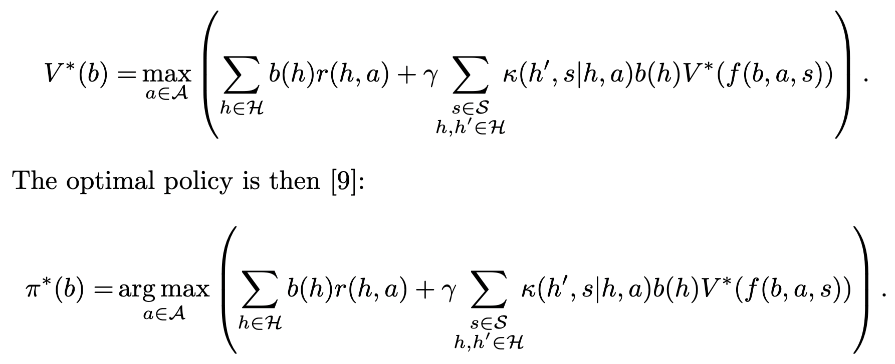
- optimal policy is function of this belief, and can be obtained via belief-MDP and optimal value function \(V^*:P\mathcal H \to \mathbb R\) on beliefs
POMDP solution
Given a POMDP with hidden state space \(\mathcal H\)
- optimal value function solves Bellman equation:
-
Moore machine that solves POMDP
Given a POMDP construct Moore machine
- choose
- \(P\mathcal H\) as internal state space
- \(\mathcal S\) as input space
- \(\mathcal A\) as output space
- \(\pi^*:P\mathcal H \to \mathcal A\) as output function
- given optimal policy \(\pi^*:P\mathcal H \to \mathcal A\)
- choosing optimal action \(a=\pi^*(b)\) we can
- turn belief update into Moore machine transition kernel:
- \(f_{\pi^*}(s,b):=f(b,\pi^*(b),s)\)
- \(\mu(b'|s,b):=\delta_{f_{\pi^*}(s,b)}(b')\)
Justified to call this a rational agent with beliefs and a goal!
Moore machine with interpretation
Yey! We got some agent! But we can find more! Some machines
- do everything necessary to specify the beliefs and actions that solve a POMDP
- but have state spaces that aren't spaces of probability distributions themselves (they are like sufficient statistics a bit)
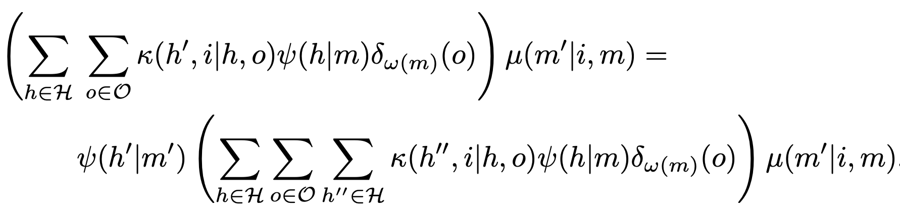
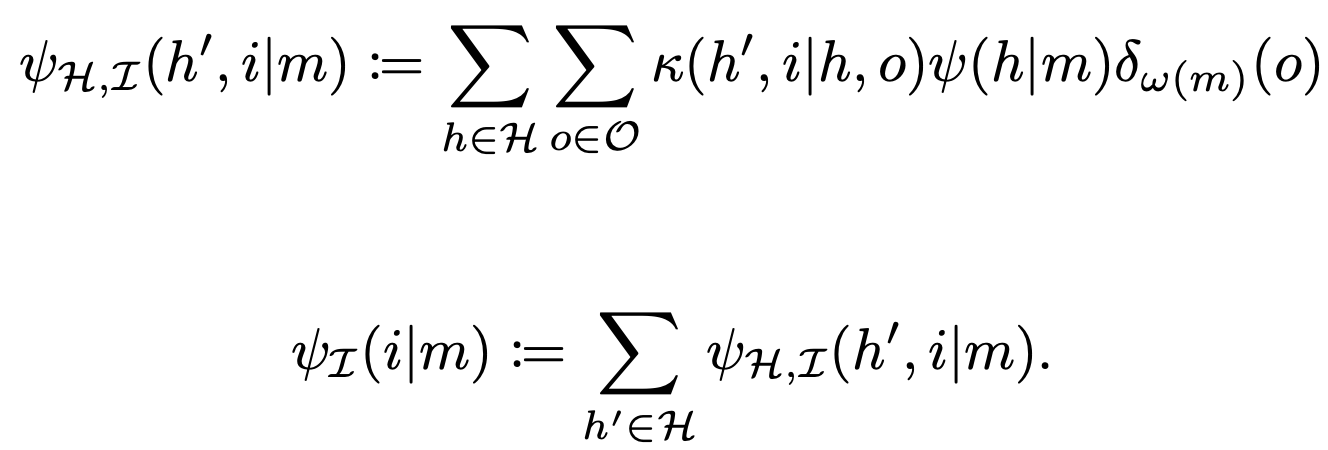
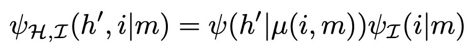
- for this we need to specify an interpretation map \(\psi:\mathcal M \to P\mathcal H\) such that the machine kernel must obey a consistency equation with respect to the POMDP transition kernel:
Simplified notation:
- specify an interpretation map \(\psi:\mathcal M \to P\mathcal H\) such that the machine kernel \(\mu\) must obey a consistency equation with respect to the POMDP transition kernel \(\kappa\)
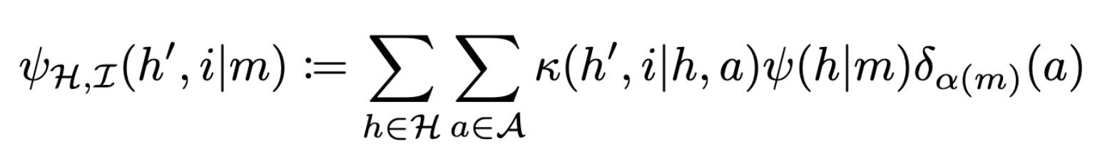
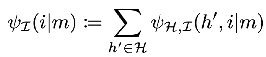
- define prior over next hidden state and input/sensor value:
- and only over next sensor value:
- then consistency means (if \(\psi_{\mathcal I}(i|m)>0\)):
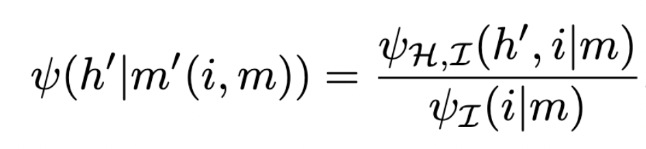
Moore machine with interpretation
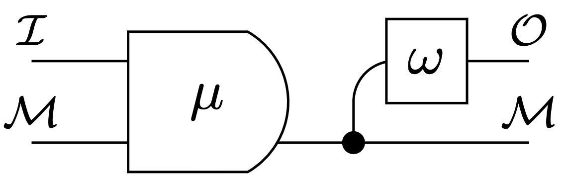
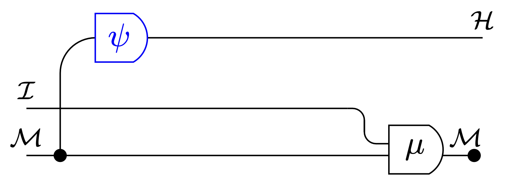
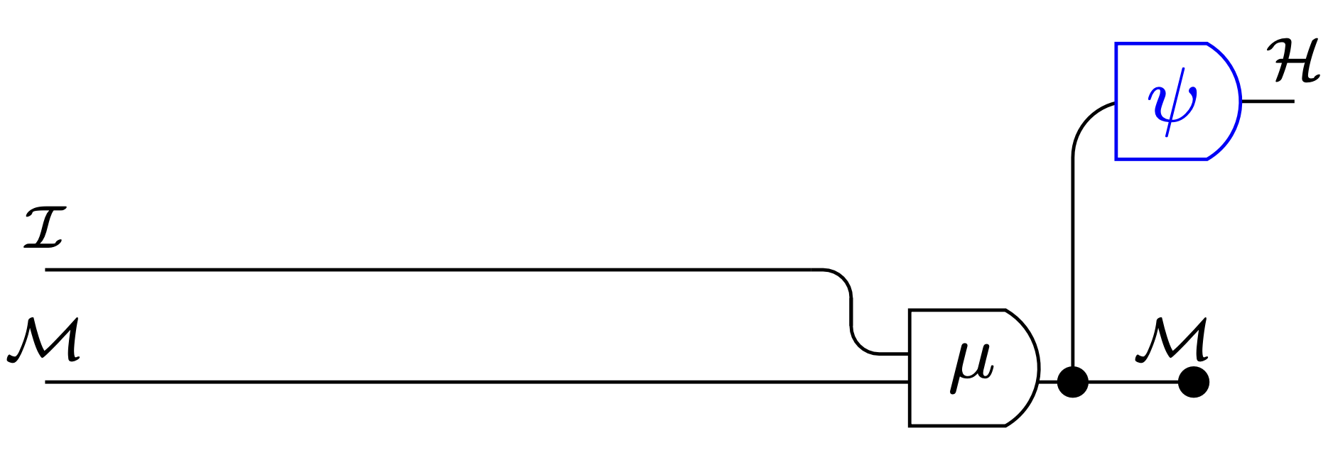
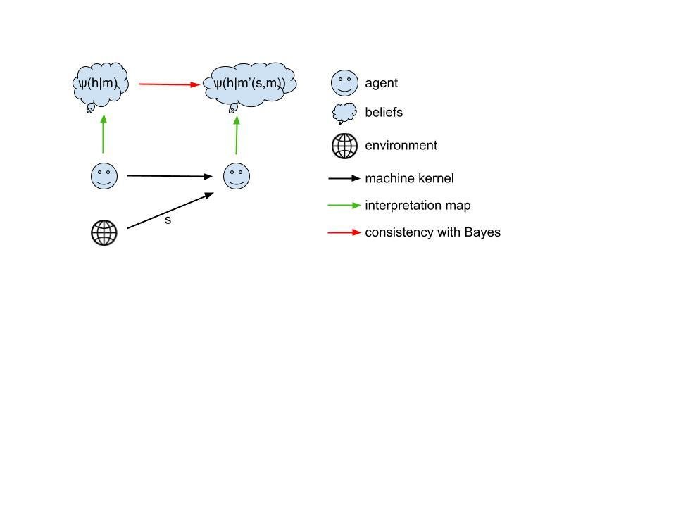
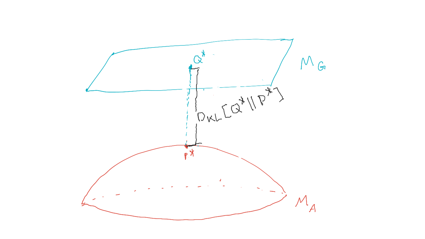
Informal image:
Moore machine with interpretation
Main statement:
Given a Moore machine a consistent interpretation as a solution to a POMDP is given by:
- a POMDP
- an interpretation map
such that
- machine kernel \(\mu\) is consistent with interpretation map \(\psi\) and POMDP transition kernel \(\kappa\)
- output function of Moore machine select optimal action:
Moore machine with interpretation
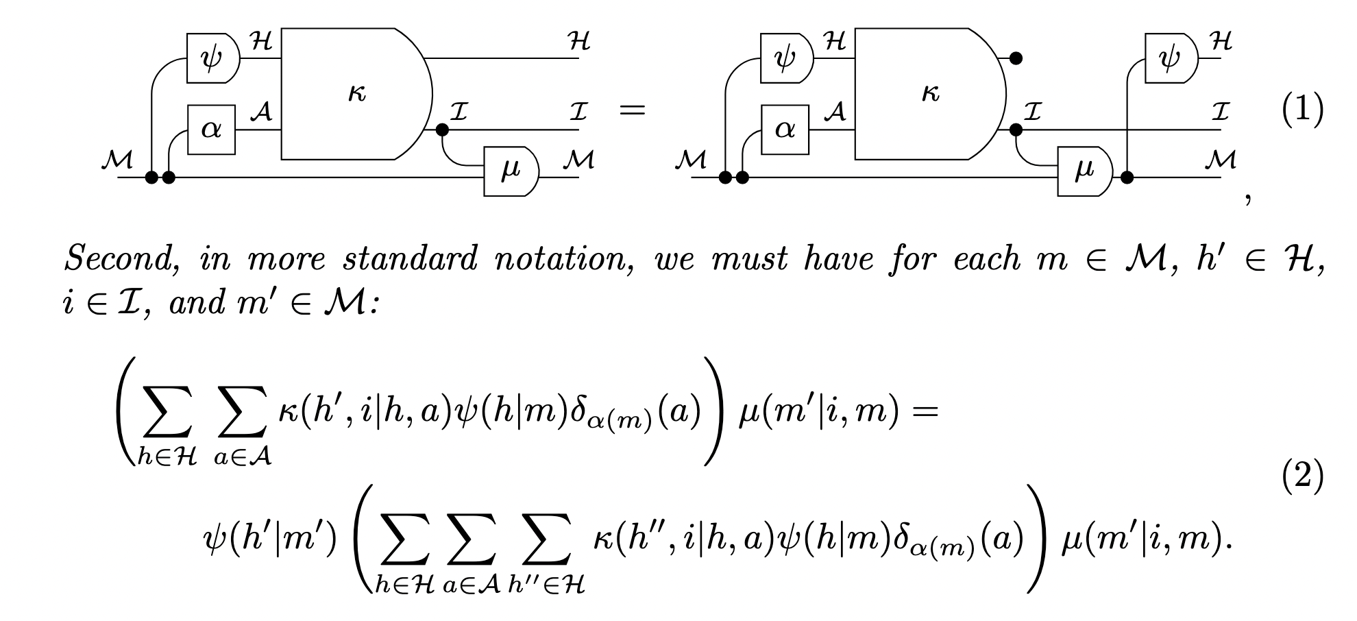
String diagram consistency
Interpreting systems a Bayesian reasoners
Recall Bayes rule (for any random variables \(A,B\)):
\[p(b\,|\,a) = \frac{p(a\,|\,b)}{p(a)} \;p(b)\]
- where
\[p(a) = \sum_b p(a\,|\,b)\;p(b)\] - if we know \(p(a\,|\,b)\) and \(p(b)\) we can compute \(p(b\,|\,a)\)
- nice.
Interpreting systems a Bayesian reasoners
Bayesian inference:
- parameterized model: \(p(x|\theta)\)
- prior belief over parameters \(p(\theta)\)
- observation / data: \(\bar x\)
- Then according to Bayes rule:
\[p(\theta|x) = \frac{p(x|\theta)}{p(x)} p(\theta)\]
Interpreting systems a Bayesian reasoners
Bayesian belief updating:
- introduce time steps \(t\in \{1,2,3...\}\)
- initial belief \(p_1(\theta)\)
- sequence of observations \(x_1,x_2,...\)
- use Bayes rule to get \(p_{t+1}(\theta)\):
\[p_{t+1}(\theta) = \frac{p(x_t|\theta)}{p_t(x_t)} p_t(\theta)\]
Interpreting systems a Bayesian reasoners
Bayesian belief updating with conjugate priors:
- now parameterize the belief
using the "conjugate prior" for model \(p(x|\theta)\)
\[p_1(\theta) \mapsto p(\theta|\alpha_1) \] - \(\alpha\) are called hyperparameters
- plug this into Bayesian belief updating:
\[p(\theta|\alpha_{t+1}) = \frac{p(x_t|\theta)}{p(x_t|\alpha_t)} p(\theta|\alpha_t)\]
where \(p(x_t|\alpha_t) := \int_\theta p(x_t|\theta)p(\theta|\alpha_t) d\theta\) - So what?
Interpreting systems a Bayesian reasoners
Bayesian belief updating with conjugate priors:
- well then: there exists a hyperparameter translation function \(f\) such that
\[\alpha_{t+1} = f(x,\alpha_t)\] - maps current hyperparameter \(\alpha_t\) and observation \(x\) to next hyperparameter \(\alpha_{t+1}\)
- but beliefs are determined by the hyperparamter!
- we can always recover them (if we want) but for computation we can forget all the probabilities!
\[p(\theta|f(x_t,\alpha_t)) = \frac{p(x_t|\theta)}{p(x_t|\alpha_t)} p(\theta|\alpha_t)\]
Interpreting systems a Bayesian reasoners
Bayesian belief updating with conjugate priors:
- so if we have a conjugate prior we can implement Bayesian belief updating with a function
\[f:X \times \mathcal{A} \to \mathcal{A}\]
\[\alpha_{t+1}= f(x,\alpha_t)\] - this is just a (discrete time) dynamical system with inputs
- Interpreting systems as Bayesian reasoners just turns this around!
Interpreting systems a Bayesian reasoners
- given discrete dynamical system with input defined by
\[\mu: S \times M \to M\]
\[m_{t+1}=\mu(s_t,m_t)\] - interpret it as implementing belief updating if find:
- interpretation map \(\psi(\theta|m)\)
- model \(\phi(s|\theta)\)
- such that the dynamical system acts like a hyperparameter translation function i.e. if:
\[\psi(\theta|\mu(s_t,m_t)) = \frac{\phi(s_t|\theta)}{(\phi \circ \psi)(s_t|m_t)} \psi(\theta|m_t)\]
Motivation / big picture
- Can we formalize the process of designing artificial agents?
Then could
- think more precisely about design choices
- classify kinds of problems in machine learning
- identify issues that hold us back from designing more interesting agents (autonomous agents / open ended agents etc)
Overview
- Designing artificial agents using probabilistic inference
- Two applications of approach:
- Designer uncertainty / problem uncertainty
- Agent uncertainty
- Recap
- Issues
Designing artificial agents
Consider designing an artificial agent where you know
- dynamics of environment \(E\) the agent will face
- sensor values \(S\) available to it
- actions \(A\) it can take
- goal \(G\) it should achieve
Then want to find
- dynamics of memory \(M\)
- selection of actions \(A\)
- that achieve the goal (or make it likely)
We show how
- express problem of designers of artificial agents face
- designers can incorporate their own uncertainty into the problem and leave it to the artificial agent to resolve it
- to ensure that the artificial agent has a Bayesian interpretation and therefore it's own well defined uncertainty
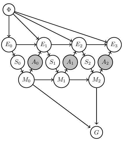
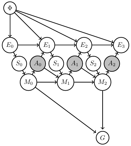
Perspective: design as planning
Designing artificial agents
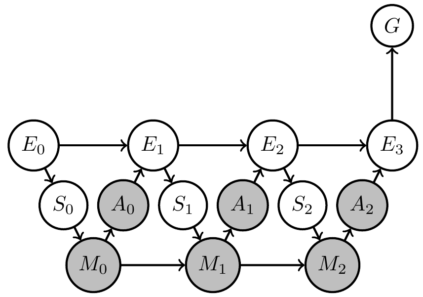
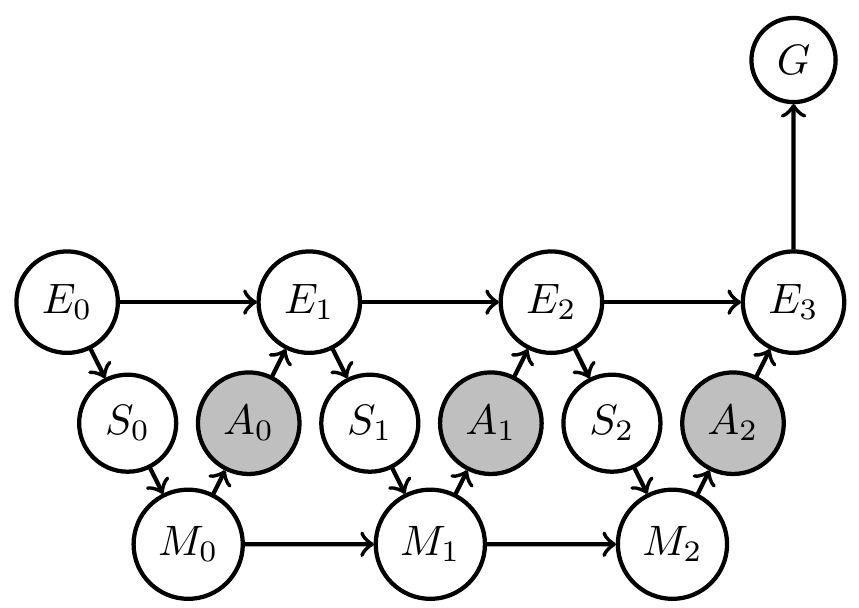
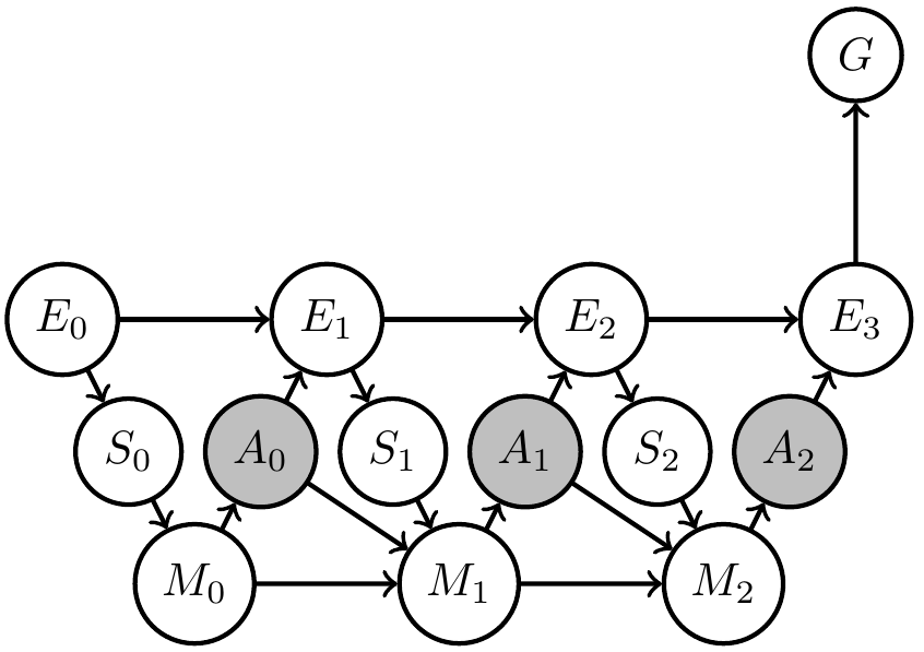
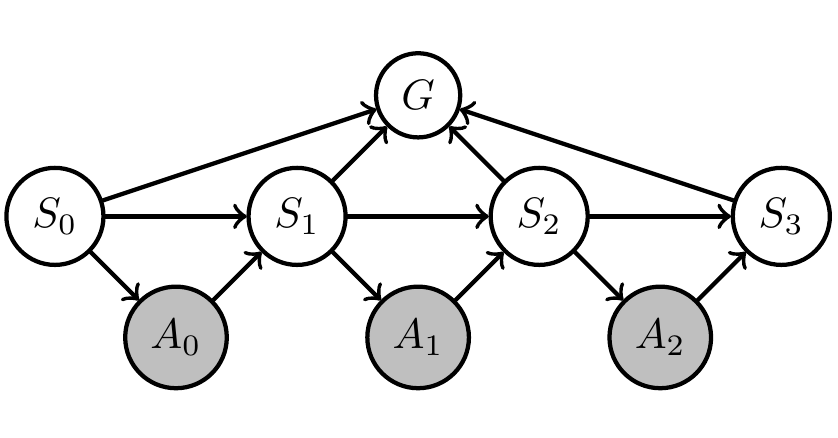
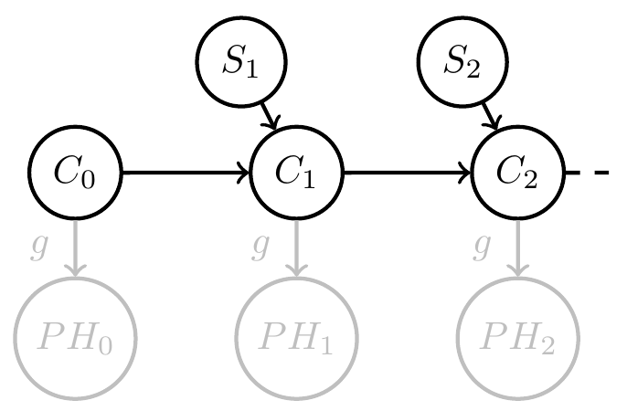
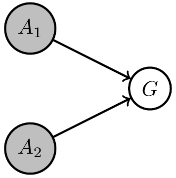
Then can (often but not always) formally represent this in Bayesian network with
- known Markov kernels (white)
- unknown Markov kernels (grey)
- goal-achieved-variable \(G\)
Designing artificial agents
- Bayesian network:
- Set of random variables \(X=(X_1,..,X_n)\)
- each variable \(X_i\) has associated
- node \(i \in V\) in a directed acyclic graph
- Markov kernel \(p(x_i|x_{\text{pa}(i)})\) defining its dependence on other variables
- Joint probability distribution factorizes according to the graph:
\[\newcommand{\pa}{\text{pa}}p(x) = \prod_{v\in V} p(x_v | x_{\pa(v)}).\]
Designing artificial agents
- Bayesian network:
- We distinguish:
- known kernels \(B\subset V\)
- unknown kernels \(U\subset V\)
- then:
\[\newcommand{\pa}{\text{pa}}p(x) = \prod_{u\in U} p_u(x_a | x_{\pa(a)}) \, \prod_{b\in B} \bar p_b(x_b | x_{\pa(b)})\]
- We distinguish:
Designing artificial agents
To find unknown kernels \(p_U:=\{p_u: u \in U\}\)
- "just" maximize probability of achieving the goal:
\[p_U^* = \text{arg} \max_{p_U} p(G=1).\]
a.k.a. planning as inference [*] - equivalent to maximum likelihood inference (can use EM algorithm etc.)
- automates design of agent memory dynamics and action selection (but hard to solve)
[*] Matthew Botvinick and Marc Toussaint. Planning as inference. Trends in cognitive sciences, 16(10):485–488, 2012.
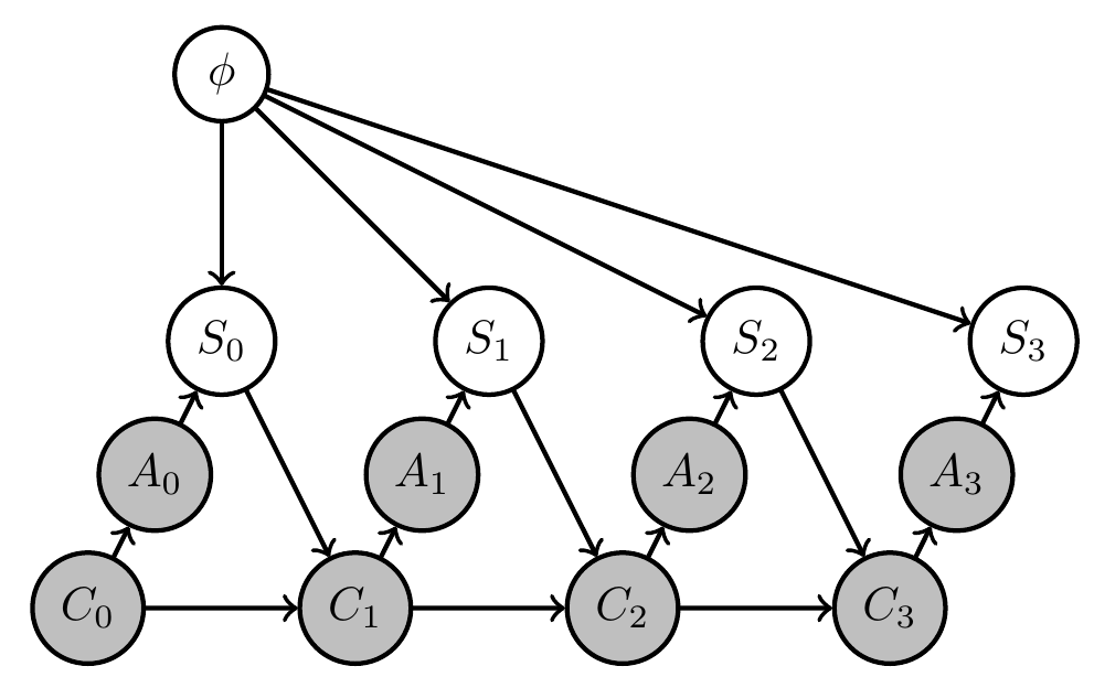
Example: 2-armed bandit
- Constant hidden "environment state" \(\phi=(\phi_1,\phi_2)\) storing win probabilities of two arms
- agent action is choice of arm \(a_t \in \{1,2\}\)
- sensor value is either win or lose sampled according to win probability of chosen arm \(s_t \in \{\text{win},\text{lose}\}\)
\[p_{S_t}(s_t|a_{t-1},\phi)=\phi_{a_{t-1}}^{\delta_{\text{win}}(s_t)} (1-\phi_{a_{t-1}})^{\delta_{\text{lose}}(s_t)}\] - goal is achieved if last arm choice results in win \(s_3=\text{win}\)
\[p_G(G=1|s_3)=\delta_{\text{win}}(s_3)\] - memory \(m_t \in \{1,2,3,4\}\) is enough to store all different results.
Example: 2-armed bandit
Two options:
- fix win probabilities to known values \[p_\Phi(\phi_1,\phi_2)=\delta_{q_1}(\phi_1) \delta_{q_2}(\phi_2)\]
- introduce uncertain probability distribution over win probabilities
Then result of planning as inference will
- ignore \(s_1,s_2\) and always choose better arm with \(a_2\) (win probabilities known to the inference algorithm)
- try both arms and choose better arm according to sensor \(s_1,s_2\) because this is better than just guessing.
Applications of this approach
Two situations:
- designer uncertain about environment dynamics
- agent supposed to deal with different environments
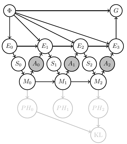
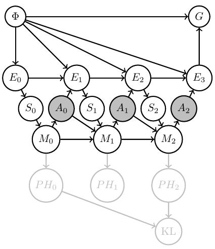
Explicitly reflect either by
- additional variable \(\phi\)
- prior distribution over \(\phi\)
Designer uncertainty
Then
- resulting agent will find out what is necessary to achieve goal
- i.e. it will trade off exploration (try out different arms) and exploitation (winning)
- comparable to meta-learning
Designer uncertainty
If we have found the agent that solves the problem
- Can we figure out what the designed agent believes about the environment?
- Maybe via an interpretation map?
- Could try to find one, but alternatively can construct agent memory to have one!
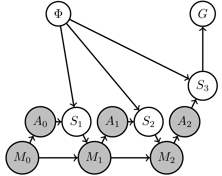
Agent uncertainty
How to fix memory dynamics \(p_M(m_t|s_t,m_{t-1})\) such that it has consistent Bayesian interpretation w.r.t chosen model
- use hyperparameter translation function of conjugate prior for the model
in 2-armed bandit:
- sensor values are Bernoulli distributed for each arm so conjugate prior is Dirichlet
- \(H=[0,1] \times [0,1]\) and assuming two win probabilities are independent choose Dirichlet prior for each: \[\psi(h||m)=\psi(h_1||m_1)\psi(h_2||m_2)\]
and agent memory counts wins and losses for each arm separately i.e. \(m_i=(m_i^{win},m_i^{loss})\) then
\[\psi(h_i||m_i):=\frac{1}{B(m_i^{win},m_i^{loss})} h_i^{m_i^{win}-1}(1-h_i)^{m_i^{loss}-1}\] - then hyperparameter translation function is
\(p_M(m_t|s_t,m_{t-1})=\delta_{m_{t-1}+\delta_}\)
Agent uncertainty
Then can make uncertainty explicit:
- choose model of causes of sensor values for agent
- fix memory dynamics \(p_M(m_t|s_t,m_{t-1})\) such that it has consistent Bayesian interpretation w.r.t chosen model
- only action kernels \(p_A(a_t|m_t)\) unknown
Agent uncertainty
Then by construction
- know a consistent Bayesian interpretation
- i.e.\ an interpretation map \(\psi:M \to PH\)
- well defined agent uncertainty in state \(m_t\) via Shannon entropy \[H_{\text{Shannon}}(m_t):=\sum_{h} \psi(h||m_t) \log \psi(h||m_t)\]
- information gain from \(m_0\) to \(m_t\) by KL divergence \[D_{\text{KL}}[m_t||m_0]:=\sum_h \psi(h||m_t) \log \frac{\psi(h||m_t)}{\psi(h||m_0)}\]
Agent uncertainty
Note:
- can then also turn this information gain into a goal to create intrinsically motivated agent
- (some trick is needed...)
Agent uncertainty
- Considered design of artificial agents as planning task
- can (sometimes) turn this into inference problem in Bayesian network
- can explicitly reflect designer's uncertainty / knowledge
- resulting agents automatically trade of exploration and exploitation
- constructing interpretable agent memory allows
- well defined (subjective) agent uncertainty and information gain
- design of agents maximizing info gain
Recap
- Why don't machine learning paper all start with a Bayesian network that shows what kind of agent they are designing?
- Can't always use Bayesian networks:
- if dependencies of variables depend on values of variables
- e.g. number of timesteps to finish task depends on actions
- Finding correct Bayesian network can be subtle
- Can't always use Bayesian networks:
- Hope to find better formalism that makes something like this possible...
Issues
Perspective: "design as inference"
Underlying perspective:
- view design of artificial agents as planning task:
- usually planning means find (own) actions that achieve a goal
- when designing an artificial agent also create a kind of "plan" but
- it will be executed by something else (e.g. computer)
- must explicitly plan "internal actions" like what to remember (memory update)
Perspective: "design as inference"
Underlying perspective:
- design of artificial agents similar to planning task:
- usually planning means find (own) actions that achieve a goal
- when designing an artificial agent to achieve a goal:
- also create a kind of "plan" but
- plan will be executed by something else (e.g. computer)
- plan must include "internal actions" like plan of what to remember (memory update)
Underlying perspective:
- known: planning can be done by probabilistic inference
\(\Rightarrow\) if we formulate agent design problems as planning problems they become inference problems
Perspective: "design as inference"
Perspective: design as planning
Underlying perspective:
- view design of artificial agents as planning task:
- use formal way to represent this planning task (planning as inference)
- gives us formal way to design agents
design as planning \(\to\) planning as inference
\(\Rightarrow\) design as inference?
General setting
Assume
- want to achieve some goal
- know:
- the environment you want to achieve it in
- actions you can take
- observations you will be able to make
Then
- planning is the process of finding actions that lead to goal
POMDPs
Formalize as POMDP:
- Known:
- goal
- environment/world state \(W\) with dynamics: \(p(w_{t+1}|w_t,a_t)\)
- observations / sensor values \(S\): \(p(s_t|w_t)\)
Planning as inference
Terminology:
- Planning:
- finding policy parameters that maximize probability of achieving a goal
- Maximum likelihood inference:
- finding model parameters that maximize probability of data
Planning as inference
What is it good for?
Automatically find a probabilistic policy to achieve a goal.
What do you need to use it?
- probabilistically specified problem!
- dynamics of environment (including influence of actions)
- inputs / sensor values / observation available to policy
- goal
Planning as inference
Combination:
- Planning as inference (PAI):
- Consider the achievement of the goal as the only available data
- ensure policy parameters are the only model parameters
- then maximizing likelihood of data maximizes likelihood of achieving the goal
\(\Rightarrow\) can use max. likelihood to solve planning!
Maximum likelihood inference
Given:
- Statistical model:
- set \(X\) of possible observations
- parameterized set \(\{p_\phi:\phi \in \Phi\}\) of probability distributions \(p_\phi(x)\) over \(X\)
- Observation \(\bar x \in X\)
Find parameter \(\phi^*\) that maximizes likelihood of the observations:
\[\phi^*=\text{arg} \max_\phi p_\phi(\bar x)\]
Maximum likelihood inference
Example: Maximum likelihood inference of coin bias
- Statistical model:
- \(X=\{(x_1,...,x_n): x_i \in \{\text{heads},\text{tails}\}\}\)
- \(\{p_\phi(x)= \phi^{c_{\text{heads}}(x)} (1-\phi)^{c_{\text{tails}}(x)}:\phi \in [0,1]\}\)
- Observation \(\bar x \in X\)
Then:
\[\phi^*=\text{arg} \max_\phi p_\phi(\bar x)=\frac{c_{\text{heads}}(\bar x)}{c_{\text{heads}}(\bar x)+c_{\text{tails}}(\bar x)}\]
Maximum likelihood inference
Example: Maximum likelihood inference of coin bias
- Statistical model:
- observations are sequences of outcomes \(X=\{(x_1,...,x_n): x_i \in \{\text{heads},\text{tails}\}\}\)
- parameterized set of distributions \(\{p_\phi:\phi \in [0,1]\}\) with
\[p_\phi(x)= \phi^{c_{\text{heads}}(x)} (1-\phi)^{c_{\text{tails}}(x)}\]
here \(c_{\text{heads}}(x)\) , \(c_{\text{tails}}(x)\) count occurrences of heads/tails in \(x\)
- Observation \(\bar x \in X\)
Find parameter \(\phi^*\) that maximizes likelihood of the observations:
\[\phi^*=\text{arg} \max_\phi p_\phi(\bar x)\]
Maximum likelihood inference
Example: Maximum likelihood inference of coin bias
- Statistical model:
- observations are sequences of outcomes \(X=\{(x_1,...,x_n): x_i \in \{\text{heads},\text{tails}\}\}\)
- parameterized set \(\{p_\phi:\phi \in \Phi=\[0,1\]\}\) with
\[p_\phi(x)= \prod_{i=1}^n \phi^{\delta_{\text{heads}}(x_i)} (1-\phi)^{\delta_{\text{tails}}(x_i)}\]
- Observation \(\bar x \in X\)
Find parameter \(\phi^*\) that maximizes likelihood of the observations:
\[\phi^*=\text{arg} \max_\phi p_\phi(\bar x)\]
Planning as inference
Note that for maximum lik
- Set of observations can be arbitrarily simple
- Set of probability distributions can be arbitrarily complicated
So we can use :
- Binary "goal-achieved-variable" with \(G=\{g,\neg g\}\) for observations
- Bayesian networks (with hidden variables) for specifying the sets of probability distributions
Planning as inference
- Problem structures as Bayesian networks:
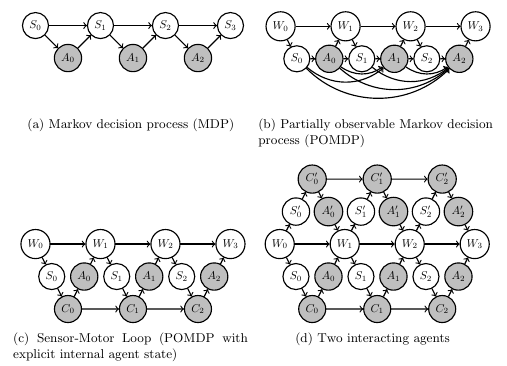
Planning as inference
Bayesian network
goal
- Represent goals and policies by sets of probability distributions:
-
goal must be an event i.e. function \(G(x)\) with
- \(G(x)=1\) if goal is achieved
- \(G(x)=0\) else.
-
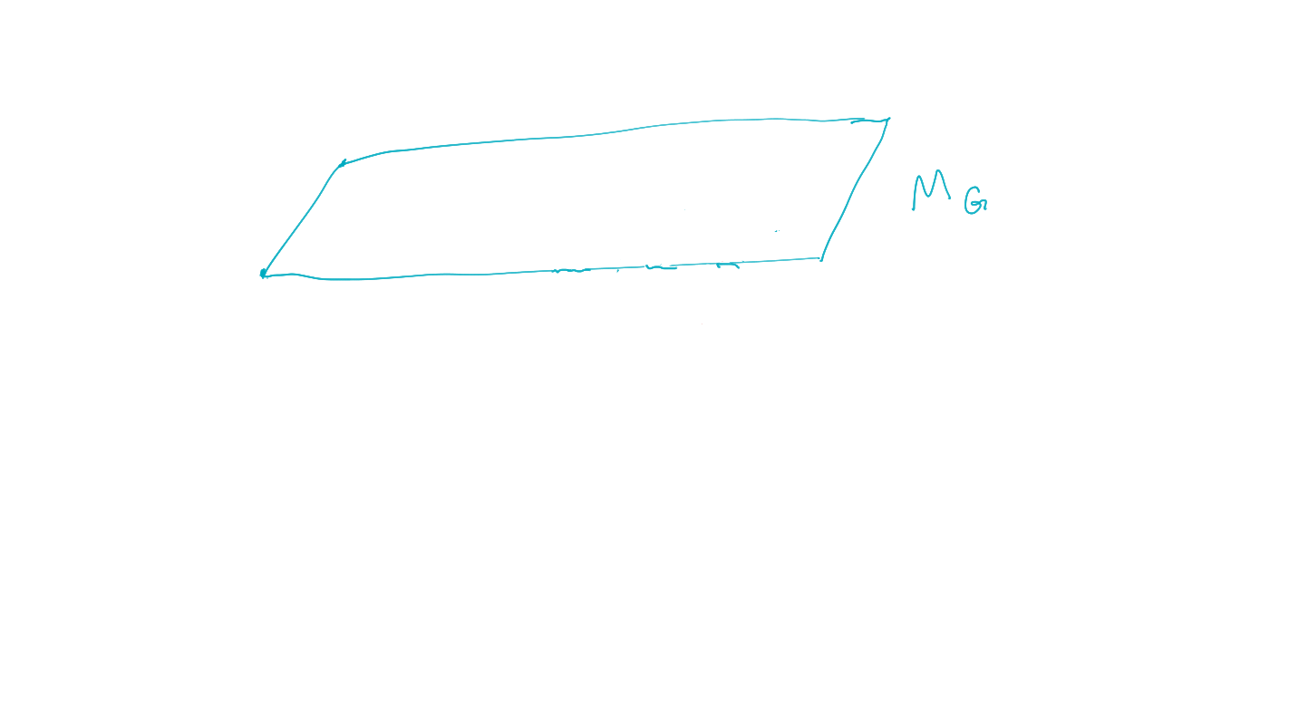
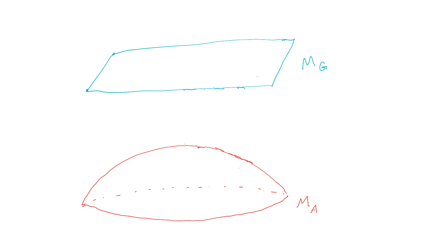
goal manifold is set of distributions where the goal event occurs with probability one:
\[M_G:=\{P: p(G=1)=1\}\]
-
goal must be an event i.e. function \(G(x)\) with
Planning as inference
- Find policies that maximize probability of goal via geometric EM algorithm:
-
planning as inference finds policy / agent kernels such that:
\[P^* = \text{arg} \max_{P \in M_A} p(G=1).\] - (compare to maximum likelihood inference)
-
planning as inference finds policy / agent kernels such that:
Bayesian network
goal
policies
Planning as inference
Practical side of original framework:
- Represent
- Planning problem structure by Bayesian networks
- Goal and possible policies by sets of probability distributions
- Find policies that maximize probability of goal via geometric EM algorithm.
Bayesian network
goal
policies
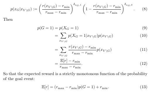
Expected reward maximization
- PAI finds policy that maximizes probability of the goal event:
\[P^* = \text{arg} \max_{P \in M_A} p(G=1).\] - Often want to maximize expected reward of a policy:
\[P^* = \text{arg} \max_{P \in M_A} \mathbb{E}_P[r]\] - Can we solve the second problem via the first?
- Yes, at least if reward has a finite range \([r_{\text{min}},r_{\text{max}}]\):
- add binary goal node \(G\) to Bayesian network and set:
\[\newcommand{\ma}{{\text{max}}}\newcommand{\mi}{{\text{min}}}\newcommand{\bs}{\backslash}p(G=1|x):= \frac{r(x)-r_\mi}{r_\ma-r_\mi}.\]
- add binary goal node \(G\) to Bayesian network and set:
Expected reward maximization
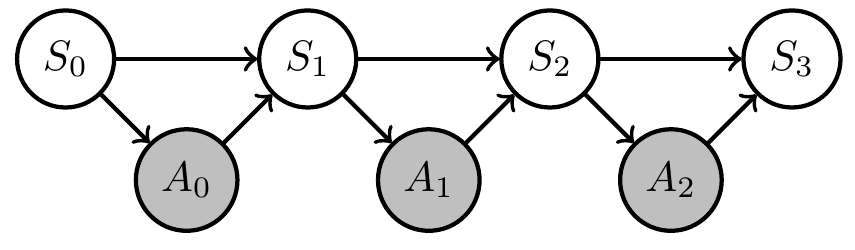
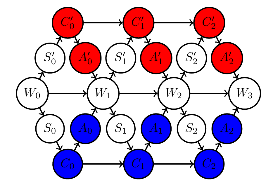
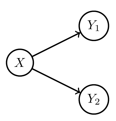
- Example application: Markov decision process
- reward only depending on states \(S_0,...,S_3\): \[r(x):=r(s_0,s_1,s_2,s_3)\]
- reward is sum over reward at each step:
\[r(s_0,s_1,s_2,s_3):= \sum_i r_i(s_i)\]
Planning as inference
- Represent goals and policies by sets of probability distributions:
-
policy is a choice of the changeable Markov kernels
\[\newcommand{\pa}{\text{pa}}\{p(x_a | x_{\pa(a)}):a \in A\}\] -
agent manifold/policy manifold is set of distributions that can be achieved by varying policy
\[\newcommand{\pa}{\text{pa}}p(x) = \prod_{a\in A} p(x_a | x_{\pa(a)}) \, \prod_{b\in B} \bar p(x_b | x_{\pa(b)})\]
-
policy is a choice of the changeable Markov kernels
Bayesian network
goal
policies
Planning as inference
- Find policies that maximize probability of goal via geometric EM algorithm:
- Can prove that \(P^*\) is the distribution in agent manifold closest to goal manifold in terms of KL-divergence
- Local minimizers of this KL-divergence can be found with the geometric EM algorithm
Bayesian network
goal
policies
Planning as inference
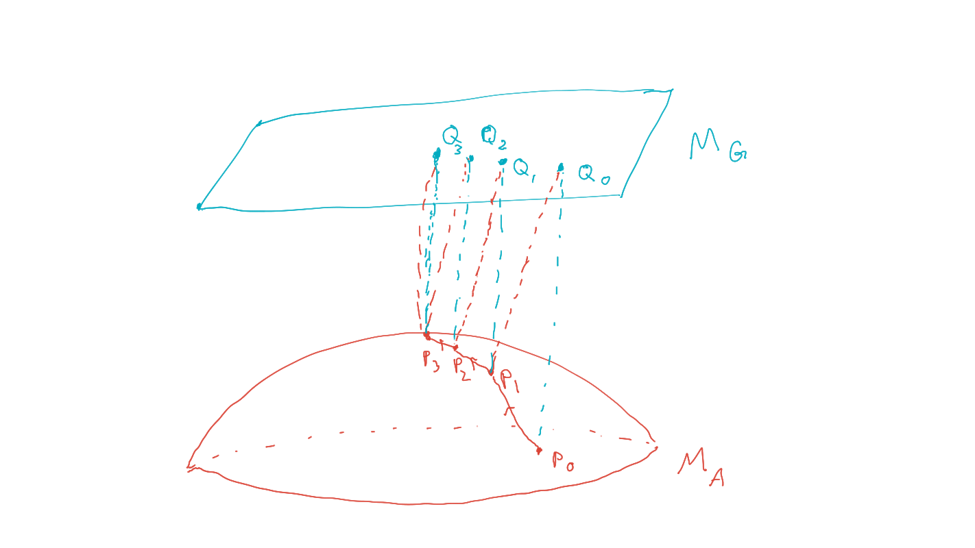
- Find policies that maximize probability of goal via geometric EM algorithm:
- Start with an initial prior, \(P_0 \in M_A\) .
- (e-projection)
\[Q_t = \text{arg} \min_{Q\in M_G} D_{KL}(Q∥P_t )\] - (m-projection)
\[P_{t+1} = \text{arg} \min_{P \in M_A} D_{KL} (Q_t ∥P )\]
Bayesian network
goal
policies
Planning as inference
- Find policies that maximize probability of goal via geometric EM algorithm:
- Equivalent algorithm using only marginalization and conditioning:
- Initial agent kernels define prior, \(P_0 \in M_A\).
- Get \(Q_t\), from \(P_t\) by conditioning on the goal: \[q_t(x) = p_t(x|G=1).\]
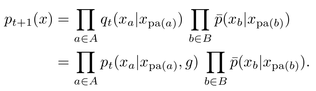
- Get \(P_{t+1}\), by replacing agent kernels by conditional distributions in \(Q_t\):
\[\newcommand{\pa}{\text{pa}} p_{t+1}(x) = \prod_{a\in A} q_t(x_a | x_{\pa(a)}) \, \prod_{b\in B} \bar p(x_b | x_{\pa(b)})\]
\[\newcommand{\pa}{\text{pa}} \;\;\;\;\;\;\;= \prod_{a\in A} p_t(x_a | x_{\pa(a)},g) \, \prod_{b\in B} \bar p(x_b | x_{\pa(b)})\]
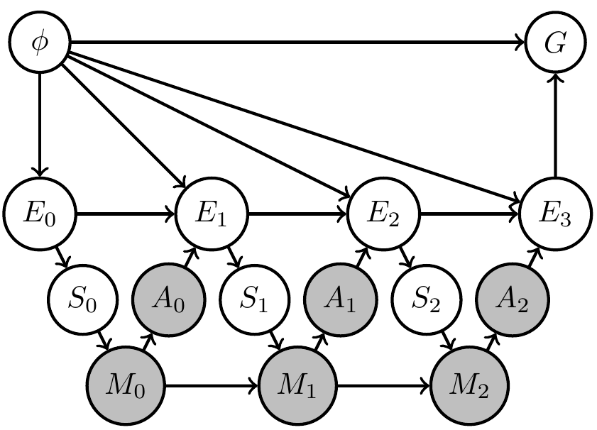
Uncertain (PO)MDP
- Assume
- (as usual) transition kernel of environment is constant over time, but
- we are uncertain about what is the transition kernel
- How can we reflect this in our setup / PAI?
- Can we find agent kernels that solve problem in a way that is robust against variation of those transition kernels?
Uncertain (PO)MDP
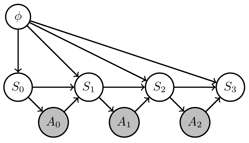
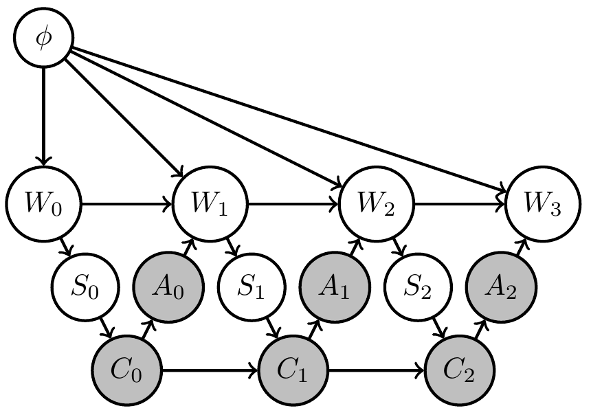
- Extend original (PO)MDP Bayesian network with two steps:
- parametrize environment transition kernels by shared parameter \(\phi\):
\[\bar{p}(x_e|x_{\text{pa}(e)}) \to \bar{p}_\phi(x_e|x_{\text{pa}(e)},\phi)\] - introduce prior distribution \(\bar{p}(\phi)\) over environment parameter
- parametrize environment transition kernels by shared parameter \(\phi\):
Uncertain (PO)MDP
- Same structure can be hidden in original network but in this way becomes a requirement/constraint
- If increasing goal probability involves actions that resolve uncertainty about the environment then PAI finds those actions!
- PAI results in curious agent kernels/policy.
Uncertain (PO)MDP
- Same structure can be hidden in original network but in this way becomes a requirement/constraint
- If increasing goal probability involves actions that resolve uncertainty about the environment then PAI finds those actions!
- PAI results in curious agent kernels/policy.
Uncertain (PO)MDP
-
Relevance for project:
- agents that can achieve goals in unknown / uncertain environments are important for AGI
- related to meta-learning
- understanding knowledge and uncertainty representation is important for agent design in general
Related project funded
- John Templeton Foundation has funded related project titled: Bayesian agents in a physical world
- Goal:
- What does it mean that a physical system (dynamical system) contains a (Bayesian) agent?
Related project funded
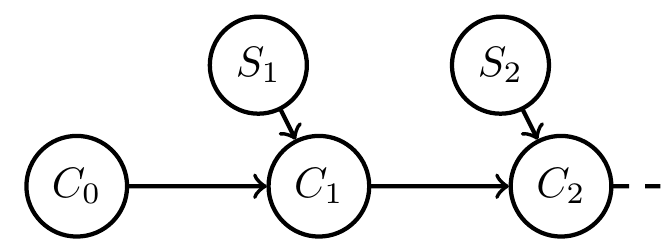
- Starting point:
- given system with inputs defined by
\[f:C \times S \to C\] - define a consistent Bayesian interpretation as:
- model / Markov kernel \(q: H \to PS\)
- interpretation function \(g:C \to PH\)
such that
\[g(c_{t+1})(h)=g(f(c_t,s_t))(h)=\frac{q(s_t|h) g(c_t)(h)}{\sum_{\bar h} q(s_t|\bar h) g(c_t)(\bar h)} \]
- given system with inputs defined by
Related project funded
- more suggestive notation:
\[g(h|c_{t+1})=g(h|f(c_t,s_t))=\frac{q(s_t|h) g(h|c_t)}{\sum_{\bar h} q(s_t|\bar h) g(\bar h|c_t)} \] - but note: \(PH_i\) are deterministic random variables and need no extra sample space
- \(H\) isn't even a deterministic random variable (what???)
Related project funded
- Take away message :
- Formal condition for when a dynamical system with inputs can be interpreted as consistently updating probabilistic beliefs about the causes of its inputs (e.g. environment)
- Extensions to include stochastic systems, actions, goals, etc. ongoing...
Related project funded
- Relevance for project
- deeper understanding of relation between physical systems and agents will also help in thinking about more applied aspects
- a lot of physical agents are made of smaller agents and grow / change their composition, understanding this is also part of the funded project and is also directly relevant for the point "dynamical scalability of multi-agent systems" in the proposal
Two kinds of uncertainty
- Designer uncertainty:
- model our own uncertainty about environment when designing the agent to make it more robust / general
- Agent uncertainty:
- constructing an agent that uses specific probabilistic belief update method
- exact Bayesian belief updating (exponential families and conjugate priors)
- approximate belief updating (VAE world models?)
- constructing an agent that uses specific probabilistic belief update method
Two kinds of uncertainty
- Designer uncertainty:
- introduce hidden parameter \(\phi\) with prior \(\bar p(\phi)\) among fixed kernels
- planning as inference finds agent kernels / policy that deal with this uncertainty
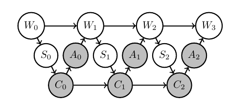
Two kinds of uncertainty
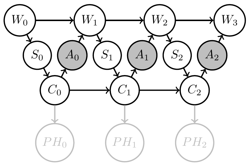
- Agent uncertainty:
- In perception-action loop:
- construct agent's memory transition kernels that consistently update probabilistic beliefs about their environment
- these beliefs come with uncertainty
- can turn uncertainty reduction itself into a goal!
- In perception-action loop:
Two kinds of uncertainty
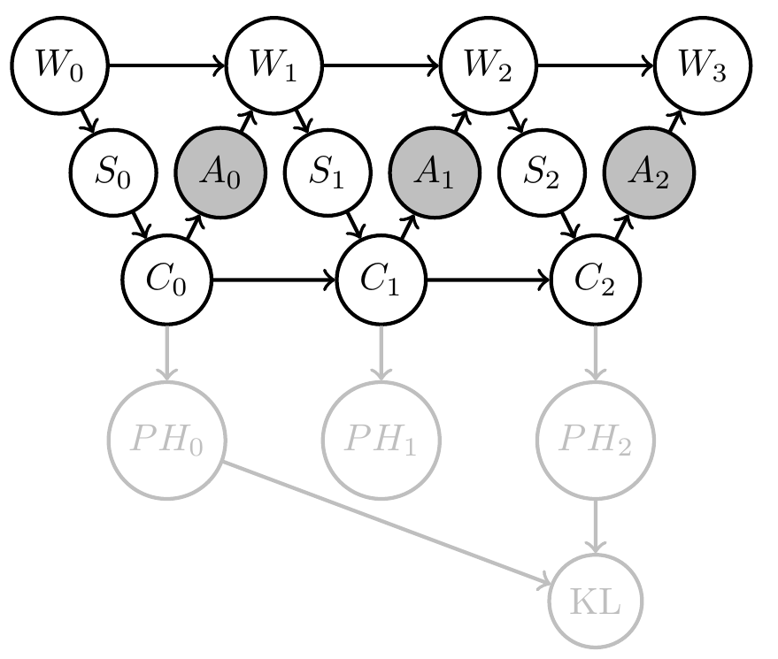
- Agent uncertainty:
- E.g: Define goal event via information gain :
\[G=1 \Leftrightarrow D_{KL}[PH_2(x)||PH_0(x)] > d\] - PAI solves for policy that employs agent memory to gain information / reduce its uncertainty by \(d\) bits
- E.g: Define goal event via information gain :
Two kinds of uncertainty
-
Relevance for project:
- taking decisions based on agent's knowledge is part of the project
Progress
- Successfully extended framework by features necessary for tackling goals of our project.
- These are discussed next:
- Expected reward maximization
- Parametrized kernels
- Shared kernels
- Multi-agent setup and games
- Uncertain (PO)MDP
- Related project funded
- Two uncertainties: designer and agent uncertainty
- Relevance for project will be highlighted
Expected reward maximization
- Relevance for project:
- reward based problems more common than goal event problems ((PO)MDPs, RL, losses...)
- extends applicability of framework
Parametrized kernels
- Often we don't want to choose the agent kernels completely freely e.g.:
- choose parametrized agent kernels
\[p(x_a|x_{\text{pa}(a)}) \to p(x_a|x_{\text{pa}(a)},\theta_a)\]
- choose parametrized agent kernels
- What do we have to adapt in this case?
- Step 3 of EM algorithm has to be adapted
Parametrized kernels
- Algorithm for parametrized kernels (not only conditioning and marginalizing anymore):
- Initial parameters \(\theta(0)\) define prior, \(P_0 \in M_A\).
- Get \(Q_t\), from \(P_t\) by conditioning on the goal: \[q_t(x) = p_t(x|G=1).\]
- Get \(P_{t+1}\), by replacing parameter \(\theta_a\) of each agent kernel with result of:

Parametrized kernels
- Relevance for project:
- needed for shared kernels
- needed for continuous random variables
- neural networks are parametrized kernels
- scalability
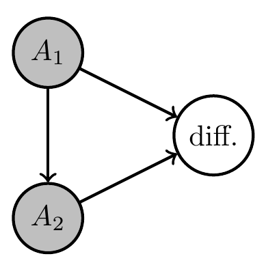
Shared kernels
- We also often want to impose the condition that multiple agent kernels are identical
- E.g. the three agent kernels in this MDP:
Shared kernels
- Introduce "types" for agent kernels
- let \(c(a)\) be the type of kernel \(a \in A\)
- kernels of same type share
- input spaces
- output space
- parameter
- then \(p_{c(a)}(x_a|x_{\text{pa}(a)},\theta_c)\) is the kernel of all nodes with \(c(a)=c\).
Shared kernels
- Example agent manifold change under shared kernels
Shared kernels
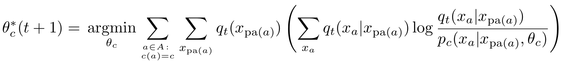
- Algorithm then becomes
- Initial parameters \(\theta(0)\) define prior, \(P_0 \in M_A\).
- Get \(Q_t\), from \(P_t\) by conditioning on the goal: \[q_t(x) = p_t(x|G=1).\]
- Get \(P_{t+1}\), by replacing parameter \(\theta_c\) of all agent kernels of type \(c\) with result of:
Proposal
- Exploit planning as inference setup to answer questions about:
-
Multiple, possibly competing goals
-
Coordination and communication from an information theoretic perspective
-
Dynamic scalability of multi-agent systems
-
Dynamically changing goals that depend on knowledge acquired through observations
-
Shared kernels
- Relevance for project:
- scalability (less parameters to optimize)
- make it possible to have
- multiple agents with same policy
- constant policy over time
Multi-agent setup
Example multi agent setups:
Two agents interacting with same environment
Two agents with same goal
Two agents with different goals
Multi-agent setup
- Note:
- In cooperative setting:
- can often combine multiple goals to single common goal via event intersection, union, complement (supplied by \(\sigma\)-algebra)
- single goal manifold
- in principle can use single agent PAI as before
- In cooperative setting:
Multi-agent setup
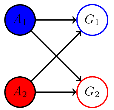
- Note:
- In non-cooperative setting:
- goal events have empty intersection
- no common goal
- multiple disjoint goal manifolds
- goal events have empty intersection
- In non-cooperative setting:
Multi-agent setup
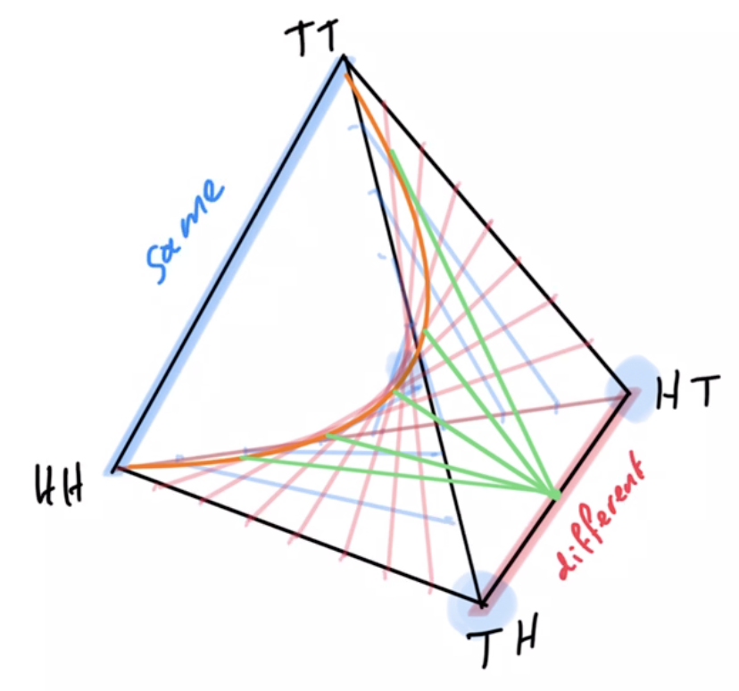
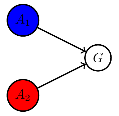
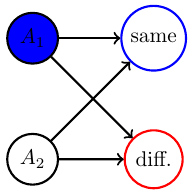
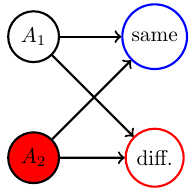
Example non-cooperative game: matching pennies
- Each player \(P_i \in \{1,2\}\) controls a kernel \(p(a_i)\) determining probabilities of heads and tails
- First player wins if both pennies are equal second player wins if they are different
Multi-agent setup
Example non-cooperative game: matching pennies
- Each player \(P_i \in \{1,2\}\) controls a kernel \(p(a_i)\) determining probabilities of heads and tails
- First player wins if both pennies are equal second player wins if they are different
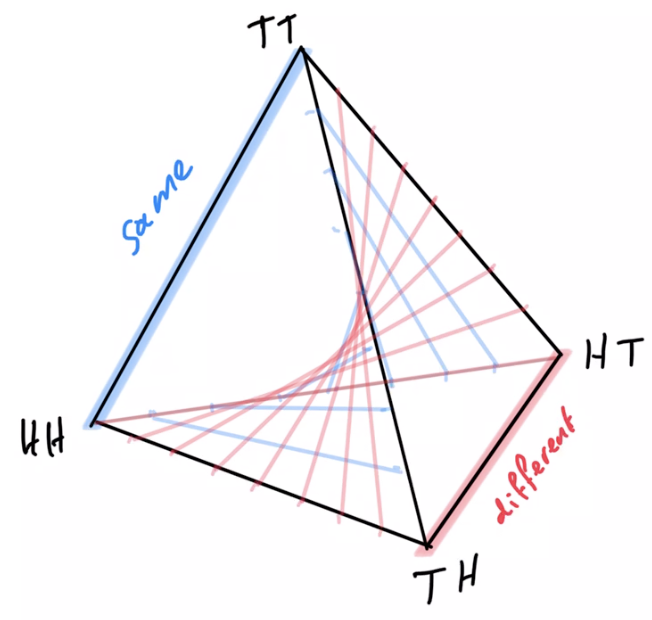
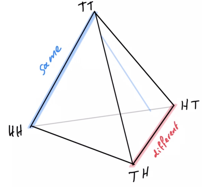
joint pdists \(p(a_1,a_2)\)
disjoint goal manifolds
agent manifold
\(p(a_1,a_2)=p(a_1)p(a_2)\)

Non-cooperative games
- In non-cooperative setting
- instead of maximizing goal probability:
- find Nash equilibria
- can we adapt PAI to do this?
- established that using EM algorithm alternatingly does not converge to Nash equilibria
- other adaptations may be possible...
- instead of maximizing goal probability:
Non-cooperative games
- Counterexample for multi-agent alternating EM convergence:
- Two player game: matching pennies
- Each player \(P_i \in \{1,2\}\) controls a kernel \(p(a_i)\) determining probabilities of heads and tails
- First player wins if both pennies are equal second player wins if they are different
- Two player game: matching pennies
Non-cooperative games
- Counterexample for multi-agent alternating EM convergence:
- Nash equilibrium is known to be both players playing uniform distribution
- Using EM algorithm to fully optimize player kernels alternatingly does not converge
- Taking only single EM steps alternatingly also does not converge
EM
EM
Non-cooperative games
- Counterexample for multi-agent alternating EM convergence
- fix a strategy for player 2 e.g. \(p_0(A_2=H)=0.2\)
Non-cooperative games
Text
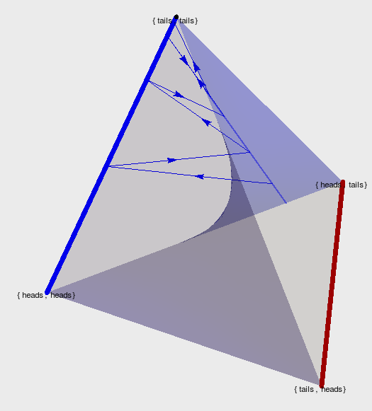
- run EM algorithm for P1
- Ends up on edge from (tails,tails) to (tails,heads)
- result: \(p(A_1=T)=1\)
- then optimizing P2 leads to \(p(A_2=H)=1\)
- then optimizing P1 leads to \(p(A_1=H)=1\)
- and on and on...
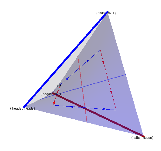
Non-cooperative games
Text
- Taking one EM step for P1 and then one for P2 and so on...
- ...also leads to loop.
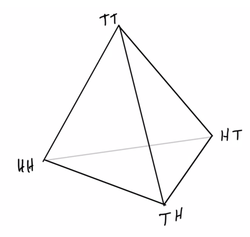
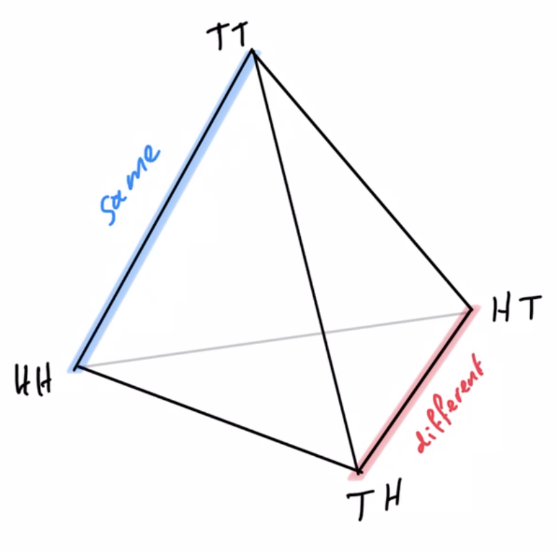
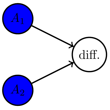
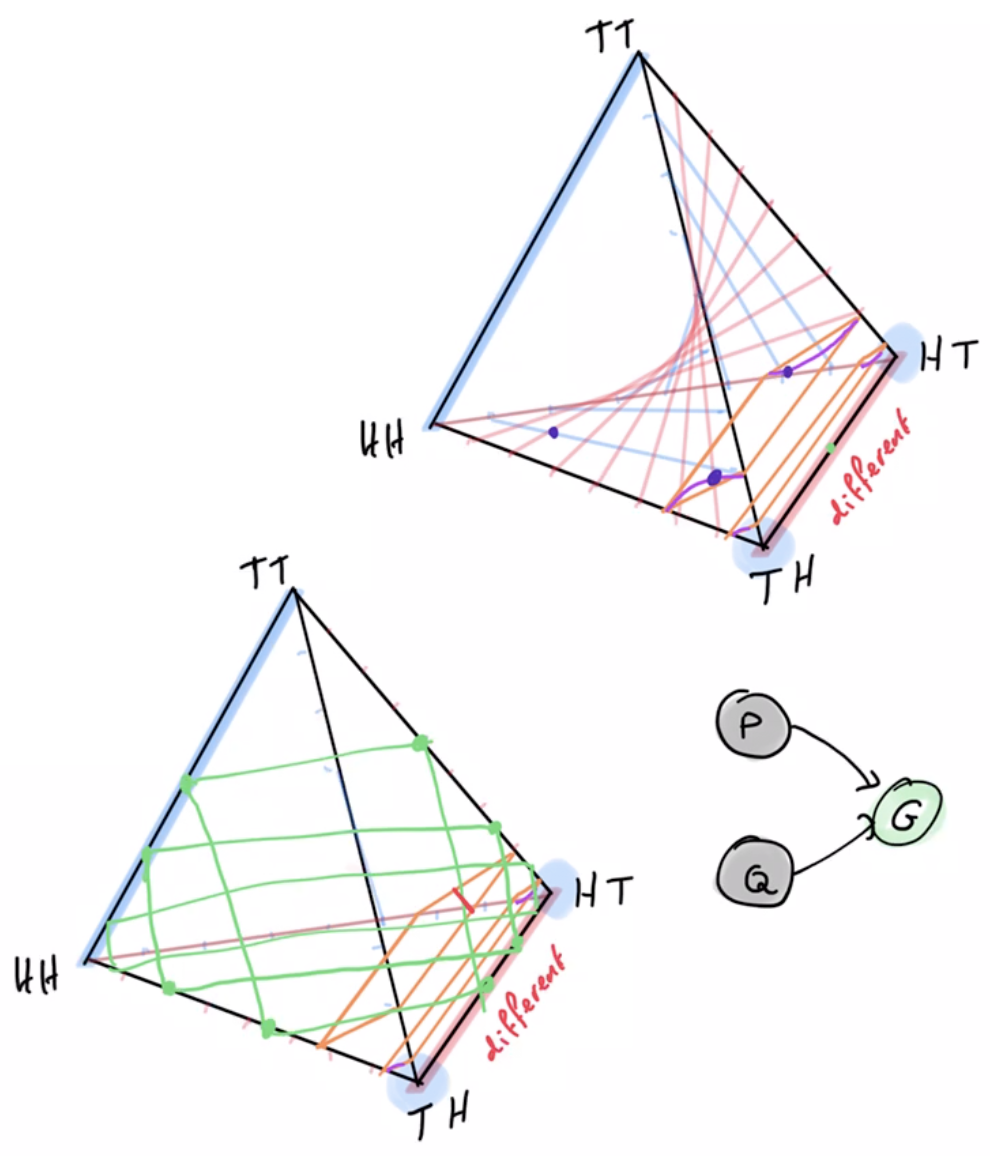
Cooperative games
- Concrete example of agent manifold reduction under switch from single agent to multi-agent to identical multi-agent setup
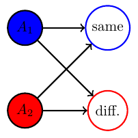
- Like matching pennies but single goal: "different outcome"
- solution: one action/player always plays heads and one always tails
- agent manifold:
- single-agent manifold would be whole simplex
- multi-agent manifold is independence manifold
- multi-agent manifold with shared kernel is submanifold of independence manifold
- Like matching pennies but single goal: "different outcome"
Cooperative games

Multi-agents and games
- Relevance to project:
- dealing with multi-agent and multiple, possibly competing goals is a main goal of the project
- basis for studying communication and interaction
- basis for scaling up number of agents
- basis for understanding advantages of multi-agent setups
Preliminary work
- Implementation of PAI in state of the art software (e.g. using Pyro)
- Planning to learn / uncertain MDP, bandit example.
- Do some agents have no interpretation e.g. the "Absent minded driver"? Collaboration with Simon McGregor.
- Design independence: some problems can be solved even if kernels are chosen independently others require coordinated choice of kernels, some are in between.
- Bayesian networks cannot change their structure dependent on the states of the contained random variables.
Preliminary work
- Implementation of PAI in state of the art software (e.g. using Pyro)
- Proofs of concept coded up in Pyro
- uses stochastic variational inference (SVI) for PAI instead of geometric EM
- may be useful to connect to work with neural networks since based on PyTorch
- For simple cases and visualizations also have Mathematica code
Preliminary work
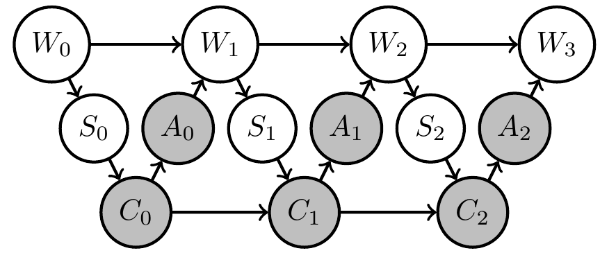
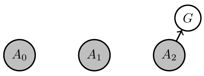
2. Planning to learn / uncertain MDP, bandit example.
- currently investigating PAI for one armed bandit
- goal event is \(G=S_3=1\)
- actions choose one of two bandits that have different win probabilities determined by \(\phi\)
- agent kernels can use memory \(C_t\) to learn about \(\phi\)
Preliminary work
- Do some agents have no interpretation e.g. the "Absent minded driver"? Collaboration with Simon McGregor.
- Driver has to take third exit
- all agent kernels share parameter \(\theta = \)probability of exiting
- optimal is \(\theta= 1/3\)
- Is this an agent even though it may have no consistent intepretation?
Preliminary work
- Design independence:
- some problems can be solved even if kernels are chosen independently
- others require coordinated choice of kernels,
- some are in between.
- Two player penny game
- goal is to get different outcomes
- one has to play heads with high probability the other has to play tails
- can't choose two kernels independently
Preliminary work
- Bayesian networks cannot change their structure dependent on the states of the contained random variables.
- Once we fix the (causal) Bayesian network it stays like that ...
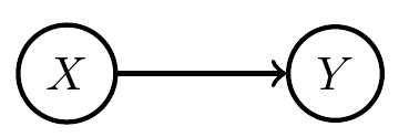
if x=1
Preliminary work
- Bayesian networks cannot change their structure dependent on the states of the contained random variables.
- Once we fix the (causal) Bayesian network it stays like that ...
if x=1
But for adding and removing agents probably needed
Preliminary work
- Bayesian networks cannot change their structure dependent on the states of the contained random variables.
- Once we fix the (causal) Bayesian network it stays like that ...
- We are learning about modern ways to deal with such changes dynamically -- polynomial functors.
Thank you for your attention!
Uncertain MDP / RL
- In RL and RL for POMDPs the transition kernels of the environment are considered unknown / uncertain
Two kinds of uncertainty
- Saw before that we can derive policies that deal with uncertainty
- This uncertainty can be seen as the "designer's uncertainty"
- But we can also design agents that have models and come with their own well defined uncertainty
- For those we can turn uncertainty reduction itself into a goal!
Two kinds of uncertainty
- Agent uncertainty:
- e.g. for agent memory implement stochastic world model that updates in response to sensor values
- then by construction each internal state has a well defined associated belief distribution \(ph_t=f(c_t)\) over hidden variables
- turn uncertainty reduction itself into a goal!
- e.g. for agent memory implement stochastic world model that updates in response to sensor values
science chat talk
By slides_martin


