Learning to Optimize
Overview
-
Motivation
-
Methods
-
Preliminary Results
Motivation
Nonlinear Optimization
Nonlinear optimization is an important problem in many domains, from control to machine learning.
$$\min_{x \in \mathbb{R}^n} f(x)$$
Training large machine learning models is time-consuming and difficult, and is one of the major obstacles towards further progress.
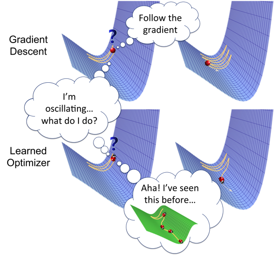
Learning to Learn
Standard algorithms for training large machine learning models use gradient information to move towards better solutions (SGD, Nesterov's accelerated gradient method, Adam, etc.)
But these standard convex optimization algorithms don't take the unique problem structure of optimizing non-convex neural networks into account. Furthermore, developing new such algorithms is difficult and time-consuming.
What if we could learn a better optimizer?
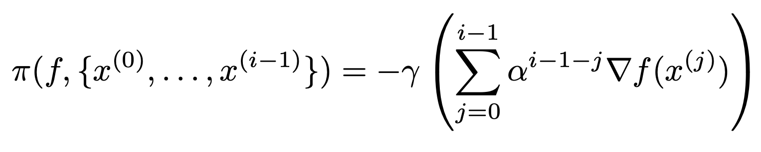
A Common Structure
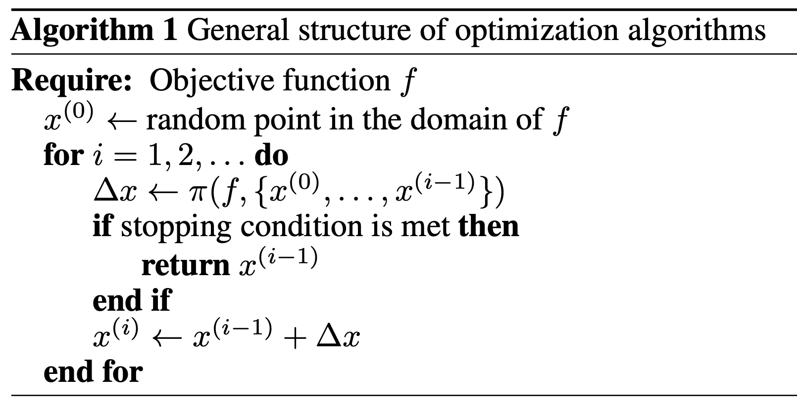
Different optimization algorithms use different \(\pi\)
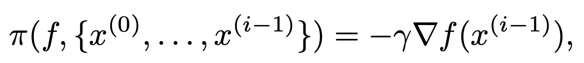
Gradient descent:
Classical momentum:
This looks awfully like a Markov Decision Process 🤔
Methods
Abstract
The 2016 paper Learning to Optimize introduced a landmark new idea to speed up the process of training neural networks: to learn the process of training itself.
The paper trained and examined performance of the method on two classes of machine learning loss functions.
They developed a method for learning a nonlinear optimization algorithms and showed that it outperforms popular hand-engineered optimization algorithms like Adam, SGD, and Nesterov's accelerated gradient method (on tiny problems).
The State Space
The dimensions of the state space encode the following information:
- Change in the objective value wrt previous iterates
$$\{f(x_i) - f(x_{i-1}), f(x_i) - f(x_{i-2}), ...\}$$
- Gradient of the objective function
$$\{\nabla f(x_i), \nabla f(x_{i-1}), ...\}$$
They keep track of only the information pertaining to the previous 25 time steps.
Rest of Environment
The action: the policy outputs a step vector \(\Delta x\) which will be used to update the current solution: $$x_{i+1} = x_i + \Delta x$$
The reward is the negative value of the objective function: $$R_i = -f(x_i)$$
Reward is undiscounted.
40 iterations allowed per optimization problem/episode.
The Algorithm
Off-policy direct policy search methods (policy gradients, actor-critic, PPO, etc.) are SOTA for high-dimensional policies like neural networks.
But they are hugely sample-inefficient. The authors identify two reasons why:
- The importance sampling ratio used in the reward estimator is often near zero, which messes with updates
- The algorithms don't know how to explore in an intelligent way. They explore randomly, bumping into parameters that lead to high reward after countless iterations
Guided Policy Search (GPS) 🥳🎉
Addressing nearly-zero IS ratio:
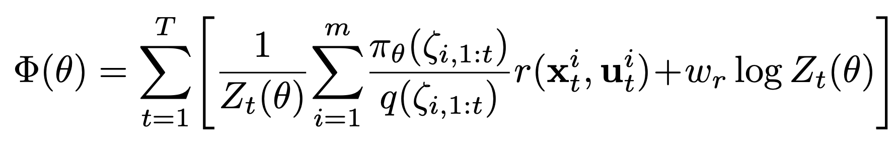
Add a regularizing term \(\log Z_t (\theta) = \sum\limits_{i=1}^m \pi_\theta (\zeta_{i, 1:t})\) that is maximized when the numerator of the IS ratio is large
Guided Policy Search (GPS) 🥳🎉
Addressing intelligent exploration:
GPS maintains two policies, \(\pi\) and \(q\).
\(q\) is a linear-gaussian policy where the optimal policy can found in closed form.
It is chosen to encourage exploration of regions with high expected reward. Specifically, \(q\) is the information projection of \(\pi\) onto the class of exponential distributions (of rewards):
$$q = \min\limits_{q \propto \exp(r(\tau))} D_{KL}(q || p)$$
Guided Policy Search (GPS) 🥳🎉
Addressing intelligent exploration cont:
It is simple to see that:
\[D_{KL}(q || p) = H(q, p) - H(q) = E_q[-\log p(\tau)] - H(q) = E_q[-r(\tau)] - H(q)\]
since \(p(\tau) \propto \exp(r(\tau))\).
So by finding this information-projection \(q\), we find a distribution that maximizes the expected reward over its trajectories and that has high entropy. High entropy means a broad distribution and better IS ratios.
Preliminary Results
Began by generating a dataset of 90 convex quadratics in 2 dimensions with eigenvalues between 1 and 5.
Also tune competing algo hyperparameters over the same dataset using Bayesian optimization.

Preliminary Results
We just used the standard PPO implementation from the stable-baselines package and will be implementing GPS over the coming days.
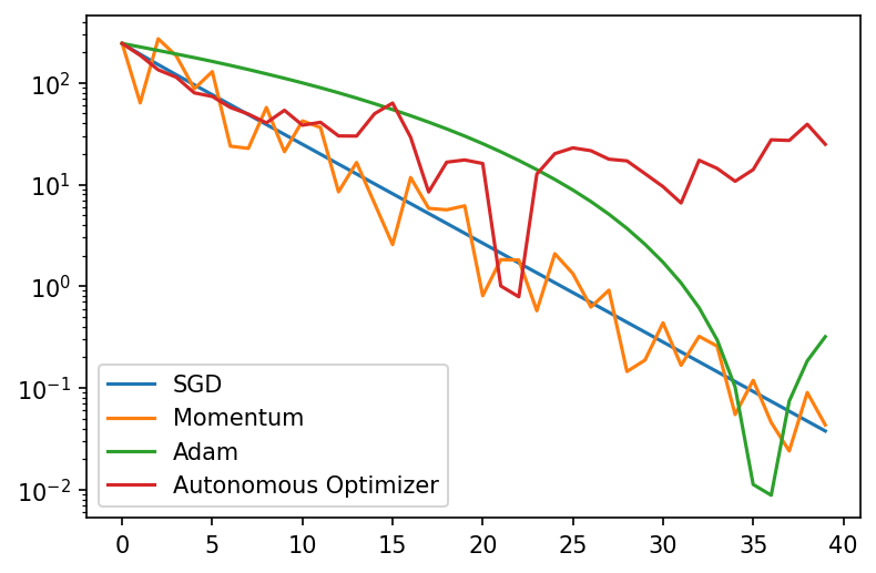
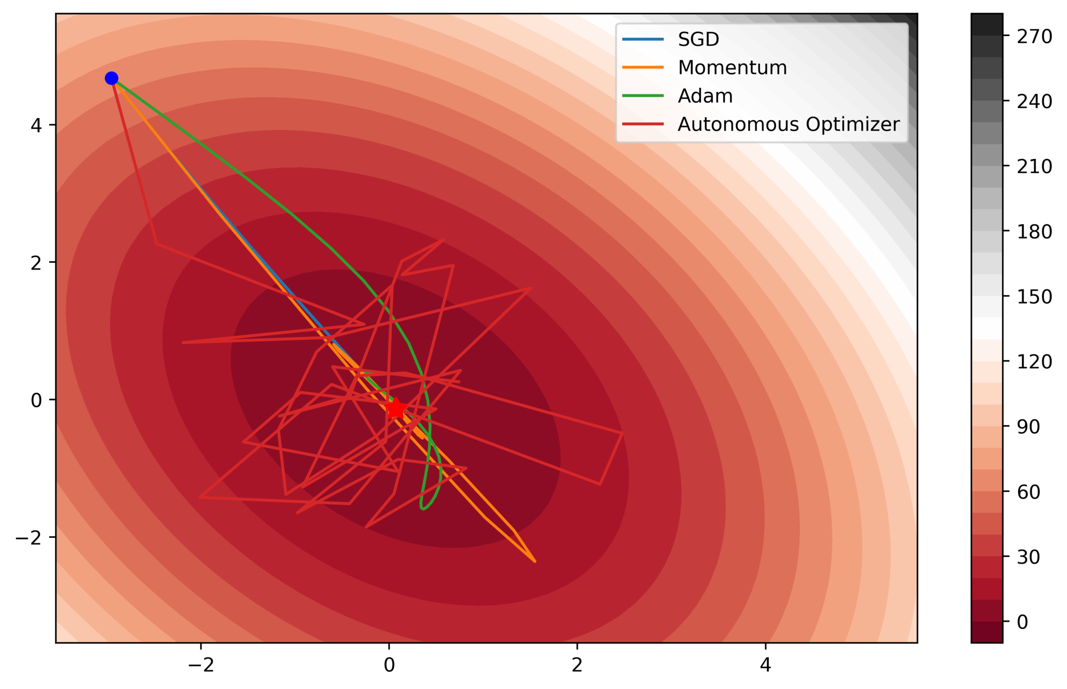
In this small problem with few iterations, all algorithms perform comparably at first, however the autonomous optimizer starts to diverge and become unstable later on. Still impressive behavior though!
Preliminary Results
Note the large step-sizes of the autonomous optimizer. This allows for fast movement towards the optimum, but it also means divergence near the minimum. We hope to address this in future versions of the code.
Questions? 🙇♂️
Learning to Optimize - Foundations of RL Final Project Presentation
By Stewy Slocum


