Supply Sense

Your go-to solution for supply chain optimization

ABOUT US

Master's in Public Policy (data track), the University of Chicago, Class of 2021

Devanshi Verma

Master's in Analytics Candidate, University of Chicago, Class of 2021

Yufei Wang

Yuanqi Mao

Master's in Public Policy (data track), the University of Chicago, Class of 2021

Agenda

Introduction
Application
Problem 1
Mixed Integer Programming
Walkthrough - Solution 1
Problem 2
Traveling Salesman Problem
Walkthrough - Solution 2
Future Work - an alternative method for TSP

Introduction

WHAT IS IT?

Supply chain management is divided broadly across the following functions

Logistics
Inventory Management and Planning
End-to-End Supply Chains
Supply Chain Execution

Introduction

COCA-COLA INDUSTRY

Agriculture and Ingredient Sourcing

The Coca Cola Company

Bottling Partners and Distributors

Consumers - Local Stores

Customers

Applications- Optimization

AMAZON'S SUPPLY CHAIN

Warehousing

Location

Size

Number of Warehouses

Delivery

Multiple Delivery Options

Technology

Robotic pick and pack

Introduction

WHAT ARE WE SOLVING?

Problem 1

We explore the challenge of allocating production demand across various facilities while minimizing the costs ensuring that the demand is met.

Problem 2

We design an optimal transportation route to improve operational efficiency while minimizing the distance.

Problem 1

BUSINESS DEFINITIONS

Problem

Optimize supply chain network to meet regional demand at the lowest cost.
Allocate production demand across various high and low capacity facilities for our client.
Evaluate whether the facility should work on low or high capacity and whether the facility should be open or closed.

Problem 1

MIXED INTEGER PROGRAMMING

Mixed Integer Programming: Some of the values are restricted to integers whereas some can be continuous like in linear programming
Where is it used?: Solve problems with discrete choices
Methods used?: Branch and bound

Problem 1

DECISION VARIABLES

STANDARD FORM

PROBLEM STATEMENT

X_{i,j} = \text{Quantity produced at i and shipped to j}

\begin{Bmatrix} Y_{i,s}=1 & \text{ if plant location i and capacity s is open} \\ Y_{i,s}=0 & \text{ if plant location i and capacity s is closed} \end{Bmatrix}

x\in Z_{+}^{n}

y\in R_{+}^{p}

Problem 1

OBJECTIVE FUNCTION

STANDARD FORM

PROBLEM STATEMENT

min \sum _{i=1}^{n} f_{is}y_{is} +\sum _{i=1}^{n}\sum _{j=1}^{m} v_{ij}x_{ij}

min \ c^{T}x + h^{T}y

f=fixed \ costs

v=variable \ costs

n=number\ of \ facilities

m = number\ of\ markets

Problem 1

CONSTRAINTS

STANDARD FORM

PROBLEM STATEMENT

Ax+By<=b

\sum _{i=1}^{n} x_{ij} = D_{j}

Y_{ih}+Y_{il}<=1

\sum _{i=1}^{n} x_{ij}<=\sum _{i=1}^{n}K_{is}y_{is}

j= 1\ to \ m

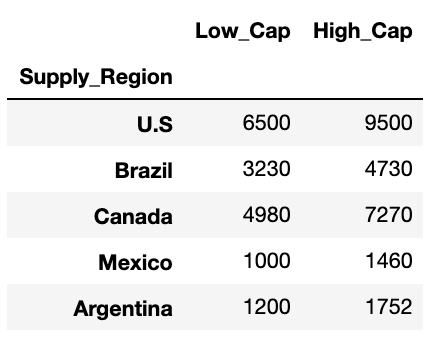
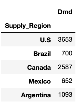
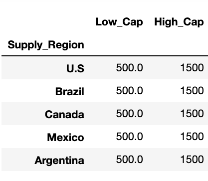
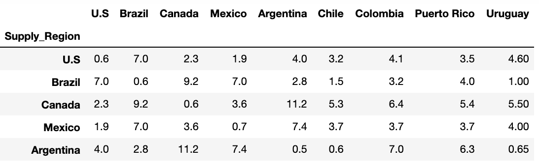
Dataset

HEAD OF DIFFERENT DATASETS USED

Fixed Cost : 9 * 2 Matrix

Variable Cost: 9 * 9 Matrix

Demand : 9 * 1 Matrix

Plant Capacity : 9 * 2 Matrix

Code

Defining Decision Variables

from pulp import *

loc=list(demand.index)
size=['Low_Cap','High_Cap']

x=LpVariable.dicts("production_", 
[(i,j) for i in loc for j in loc],
lowBound=0,upBound=None,
cat='Continuous')
    
y=LpVariable.dicts("plant_", 
[(i,s) for i in loc for s in size],
cat='Binary')

Python

Julia

using JuMP, GLPK
newModel = Model(GLPK.Optimizer)
@variable(newModel, 
0 <= x[i=1:9,j=1:9])   
@variable(newModel, 
0 <= y[i=1:9,s=1:2] <= 1, Int)

Code

Defining Objective Function

model += 
(lpSum([fix_cost.loc[i,s] * y[(i,s)] 
for s in size for i in loc])
+ lpSum([var_cost.loc[i,j] * x[(i,j)] 
for i in loc for j in loc]))

Python

Julia

total_cost = 0
for i = 1:9 
for j = 1:9
total_cost += var_cost[i,j] * x[i,j]  
print("\nvar_cost\n", var_cost[i,j] * x[i,j]) 
end
    
for s = 1:2
total_cost += fix_cost[i,s] * y[i,s]  
print("\nfix_cost\n", fix_cost[i,s] * y[i,s])
end
end

@objective(newModel, Min, total_cost)

Code

Defining Constraints

for j in loc:
model += 
lpSum([x[i,j] for i in loc]) 
== 
demand.loc[j,'Dmd']
    
for i in loc:
model += 
lpSum([x[(i, j)] for j in loc]) 
<= lpSum([cap.loc[i,s] * y[i,s] 
for s in size])
    
for i in loc:
model +=  
y[i,'High_Cap']+ y[i,'Low_Cap'] <= 1

Python

Julia

for j = 1:9
@constraint(newModel, 
sum(x[i,j] for i=1:9) == dmd[j]) 
   
for i = 1:9
@constraint(newModel, sum(x[i,j] 
for j=1:9)
<= sum(cap[i, s] * y[i, s] for s=1:2)) 
end

for i = 1:9
@constraint(newModel, sum(y[i,s] for s=1:2) <= 1) 
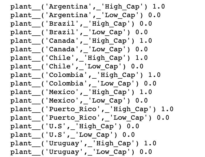
end

Result

Optimized Solution - Y

Python

Julia

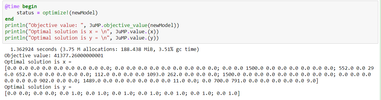
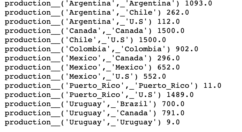
Result

Optimized Solution - x

Python

Julia

Code

Generating Maps

from geopy.geocoders import Nominatim
geolocator=Nominatim(user_agent="Optimization_Project")
a['Lat']=a['location'].apply(lambda x: geolocator.geocode(x).latitude)
a['Long']=a['location'].apply(lambda x: geolocator.geocode(x).longitude)

import folium
base_map2=folium.Map(location=[19.432630, -99.133178], zoom_start=2,tiles='cartodbpositron')
for idx, row in a.iterrows():
    location=[row['Lat'],row['Long']]
    if row['status']==1:
        popup= '<strong>'+"OPEN"+"\n"+"\n"+row['capacity']+'</strong>'
        marker=folium.Marker(location,popup=popup,icon=folium.Icon(color='green'))
    else:
        popup= '<strong>'+row['location']+'</strong>'
        marker=folium.Marker(location,popup=popup,icon=folium.Icon(color='blue'))
    marker.add_to(base_map2)

Python

Result

Cost Reduction of 60 %

model_min=LpProblem("Capacitedplantlocation",LpMinimize)
model_max=LpProblem("Capacitedplantlocation",LpMaximize)

min_value=pulp.value(model_min.objective)
max_value=pulp.value(model_max.objective)

print("the improvement is: {} %".format(((max_value-min_value)/max_value)*100))

Problem 2

Problem

Shift from operational level to supply & delivery
Optimize delivery path to traverse all regions with demand at the shortest path.

BUSINESS DEFINITIONS

Problem 2

TRAVELING SALESMAN PROBLEM

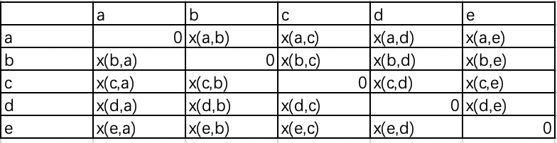
Traveling Salesman Problem: Given a series of midpoints and their corresponding distance matrix, what is the shortest path that traverses all midpoints and go back to the origin?
Where is it used?: TSP is generally an NP problem, and the solution is widely used in operations and computer science.
Methods used?: many variants including Branch & Bound, DP. But at the end of the day, the complete solution of TSP would require enumerating certain possibilities that increase together with the number of nodes, so it is a Non-Deterministic Polynomial Problem.

Problem 2

OBJECTIVE FUNCTION

PROBLEM STATEMENT

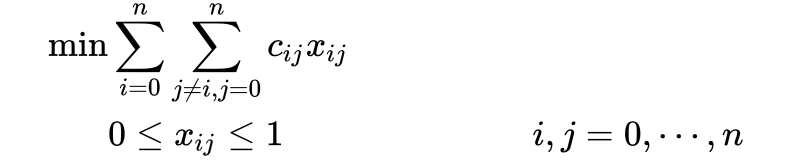
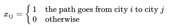
c_{ij} :\space distance \space to \space travel \space from \space place \space i \space to \space place j

Problem 1

DATA INPUT

GOOGLE GEOCODE API
GOOGLE DISTANCE MATRIX

DATA SOURCE

INPUT MATRIX

Dynamic Programming Solution

WALKING THROUGH DP SOLUTION

General Approach (Enumeration)

Dynamic Programming & Recursion

Time cost would be exponential

Introduce resource explosion

g(a,\{b,c,d,e\})=min_{k\in \{b,c,d,e\}}\{c_{ak}+g(k,\{b,c,d,e\}-\{k\})\}

g(i,s)=min_{k\in s}\{c_{ik}+g(k,s-\{k\})\}

bottom-up approach: start from root; level up with either child node that has the minimum distance on its level

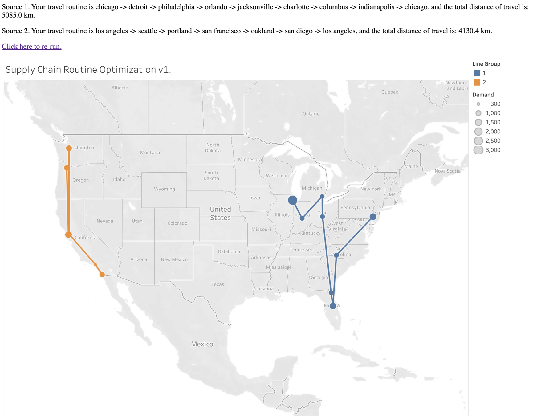
Web Demo

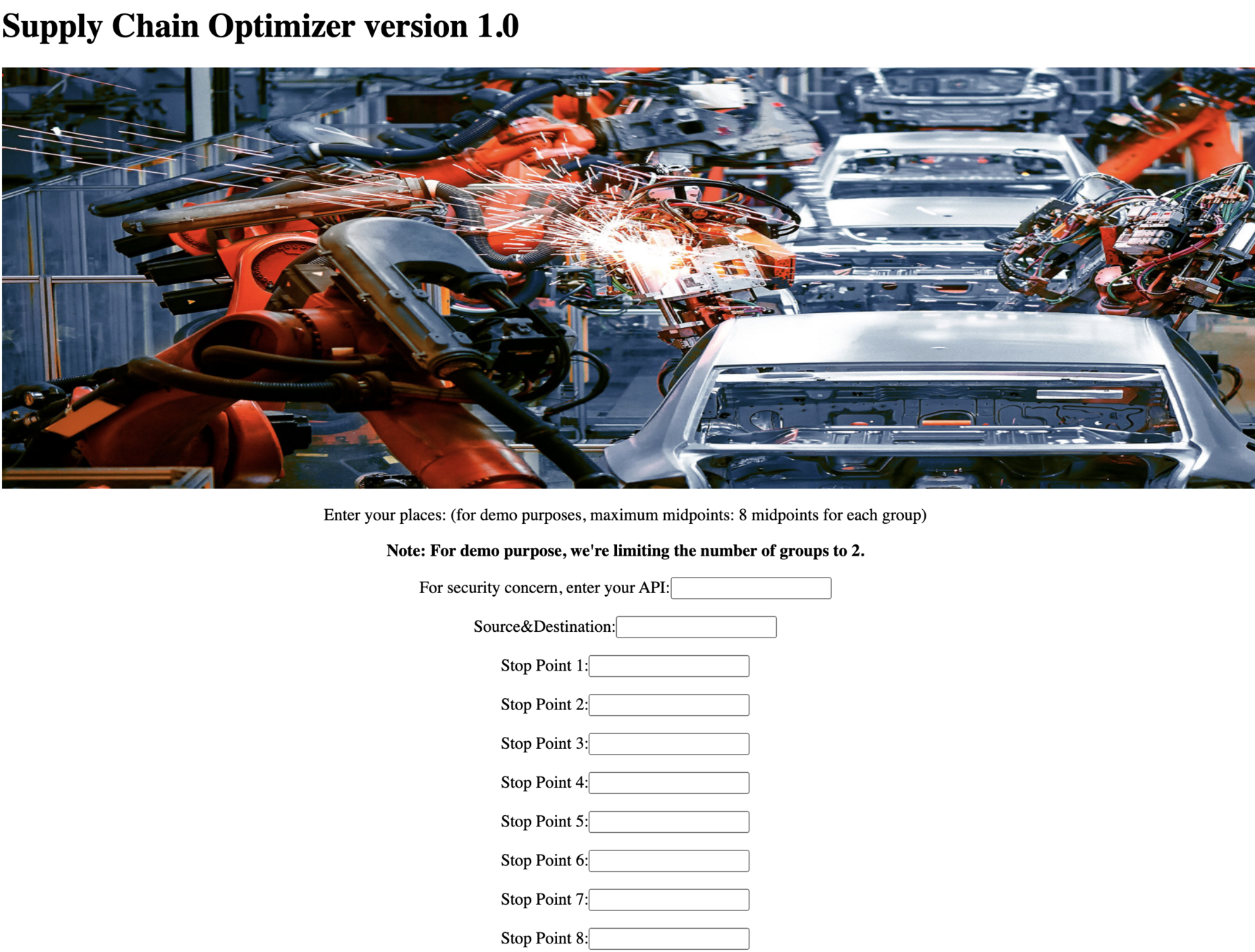
INTERACTIVE FEATURES FOR TSP SOLUTION IN SUPPLY CHAIN ANALYTICS

Web Demo

INTERACTIVE FEATURES FOR TSP SOLUTION IN SUPPLY CHAIN ANALYTICS

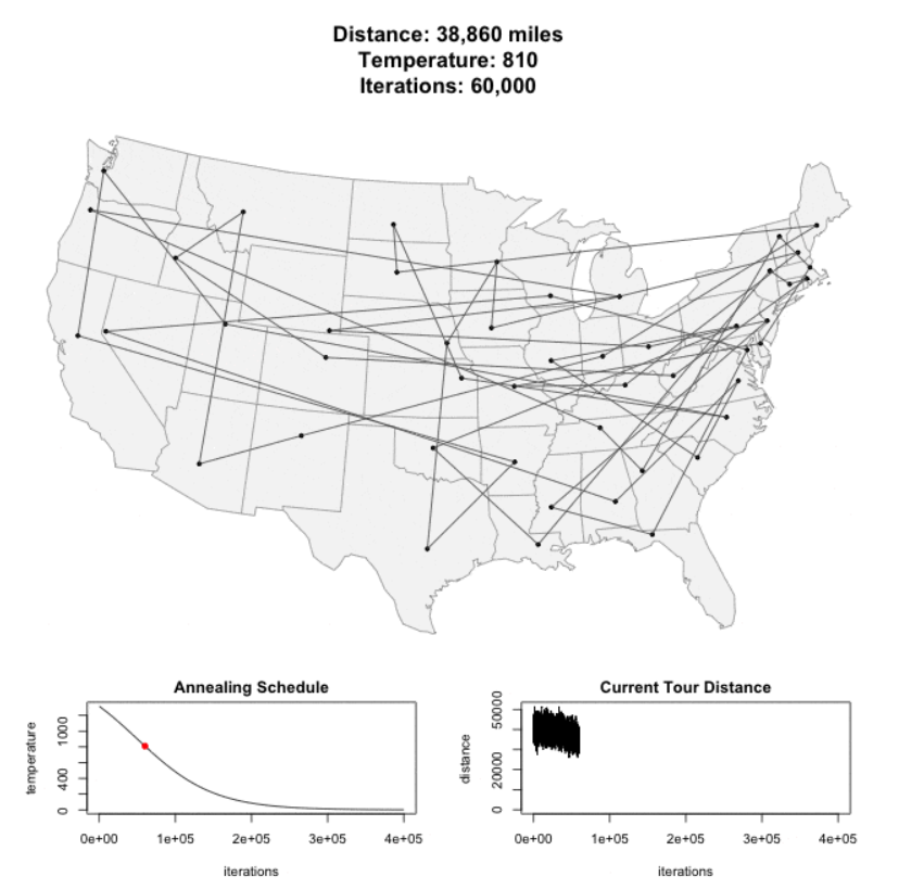
TSP - Simulated Annealing Algorithm

The method models the physical process of heating a material and then slowly lowering the temperature to decrease defects, thus minimizing the system energy.

TSP - Simulated Annealing Algorithm

The method models the physical process of heating a material and then slowly lowering the temperature to decrease defects, thus minimizing the system energy.

The algorithm is basically hill-climbing except instead of picking the best move, it picks a random move. If the selected move improves the solution, then it is always accepted. Otherwise, the algorithm makes the move anyway.

At time T, the probability of Energy change(dE) is expressed as:

P(dE) = exp( dE/(kT) )
The higher the temperature, the greater probability of Energy change.

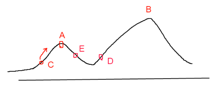
Simulated Annealing Example

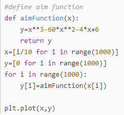
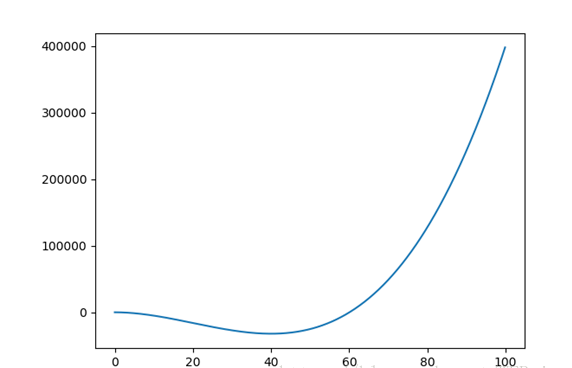
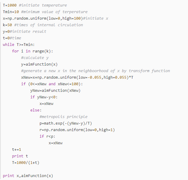
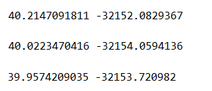
Temperature is decreased by 1000/(1+t)

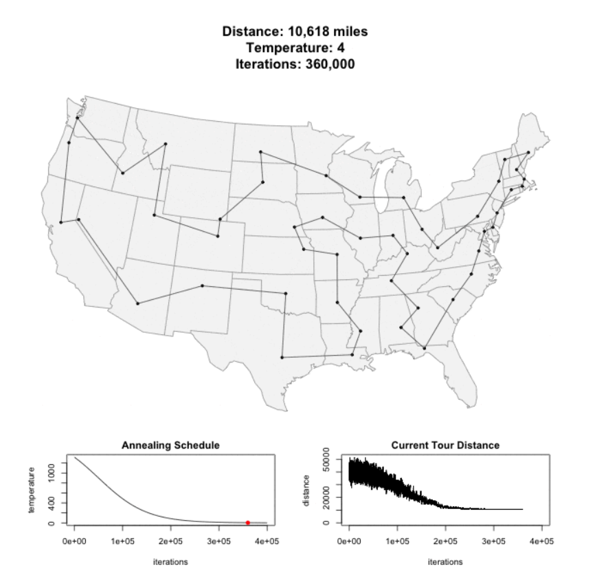
Simulated Annealing in TSP

Step 1: Start with a random tour through the selected cities.

Step 2: Pick a new candidate tour at random from all neighbors of the existing tour.

Step 3:If the candidate tour is better than the existing tour, accept it as the new tour.

Step 4:If the candidate tour is worse than the existing tour, still maybe accept it, according to some probability. The probability of accepting an inferior tour is a function of how much longer the candidate is compared to the current tour, and the temperature of the annealing process.

Step 5: Go back to step 2 and repeat many times, lowering the temperature a bit at each iteration, until you get to a low temperature and arrive at your (hopefully global, possibly local) minimum

Supply Sense

ABOUT US

Agenda

Introduction

Introduction

Applications- Optimization

Introduction

Problem 1

Problem 1

Problem 1

Problem 1

Problem 1

Dataset

Code

Code

Code

Result

Result

Code

Result

Problem 2

Problem 2

Problem 2

Problem 1

Dynamic Programming Solution

Web Demo

Web Demo

TSP - Simulated Annealing Algorithm

TSP - Simulated Annealing Algorithm

Simulated Annealing Example

Simulated Annealing in TSP

Thank You!

Optimzation-Final-Project

Optimzation-Final-Project

Devanshi Verma

Supply Sense

ABOUT US

Agenda

Introduction

Introduction

Applications- Optimization

Introduction

Problem 1

Problem 1

Problem 1

Problem 1

Problem 1

Dataset

Code

Code

Code

Result

Result

Code

Result

Problem 2

Problem 2

Problem 2

Problem 1

Dynamic Programming Solution

Web Demo

Web Demo

TSP - Simulated Annealing Algorithm

TSP - Simulated Annealing Algorithm

Simulated Annealing Example

Simulated Annealing in TSP

Thank You!

Optimzation-Final-Project

More from Devanshi Verma