


Vedant Puri
PhD student at Carnegie Mellon University
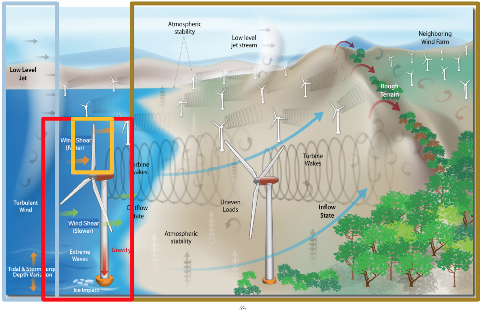
Mesosphere
Wind farm
Turbine
Blade
1
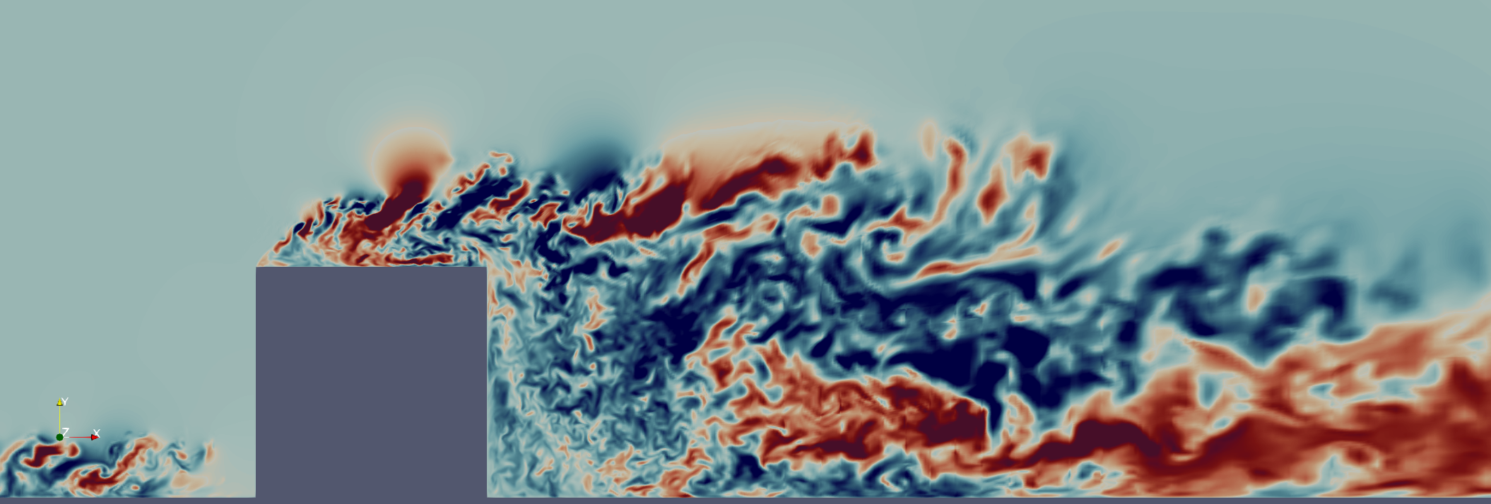
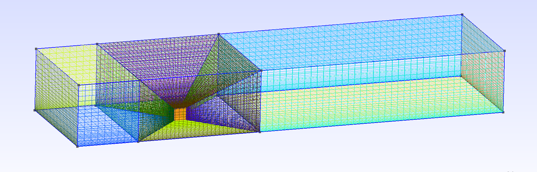
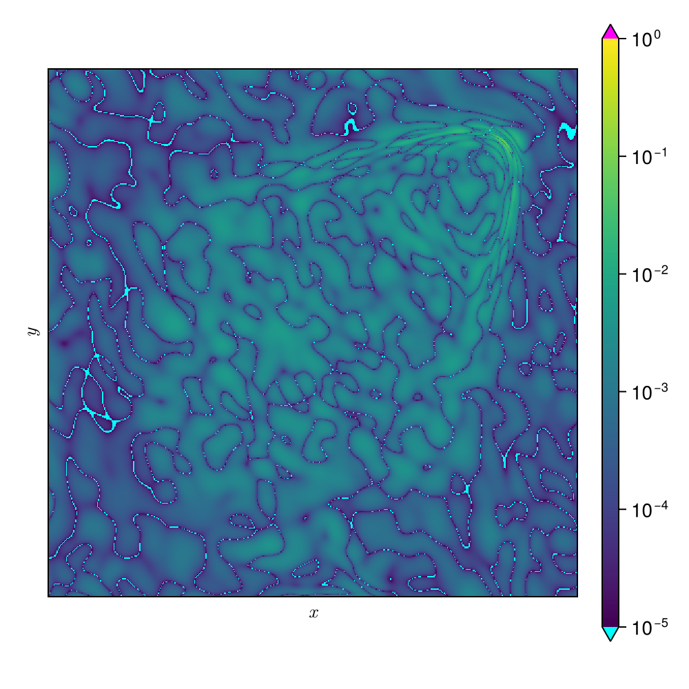
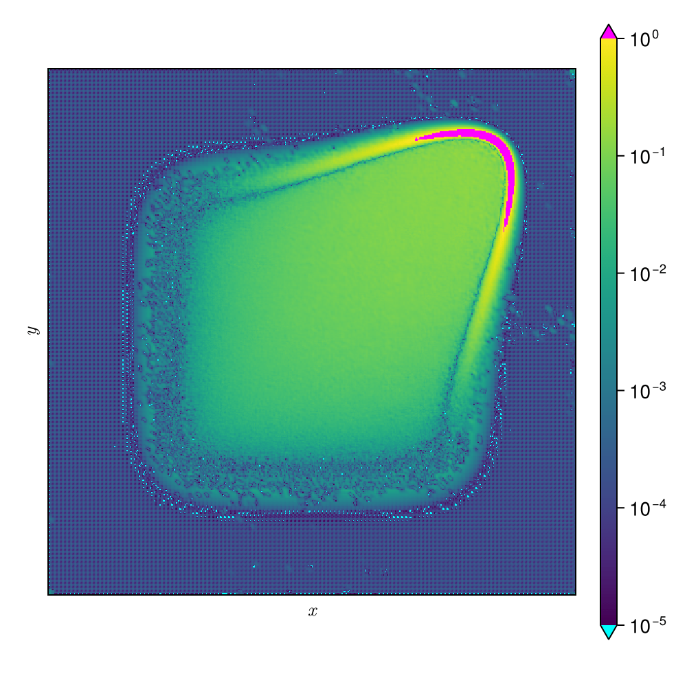
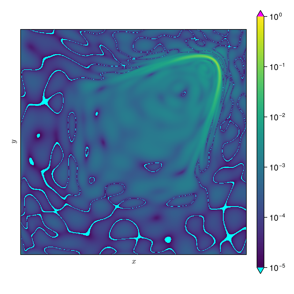
Navier-Stokes Equations
(Flow past bluff body \( Re = 3900 \))
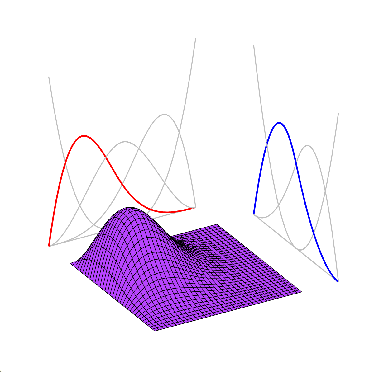
Need high quality function representation over (complex) geometry
Main operations: \(\nabla, \, \int_\Omega\)
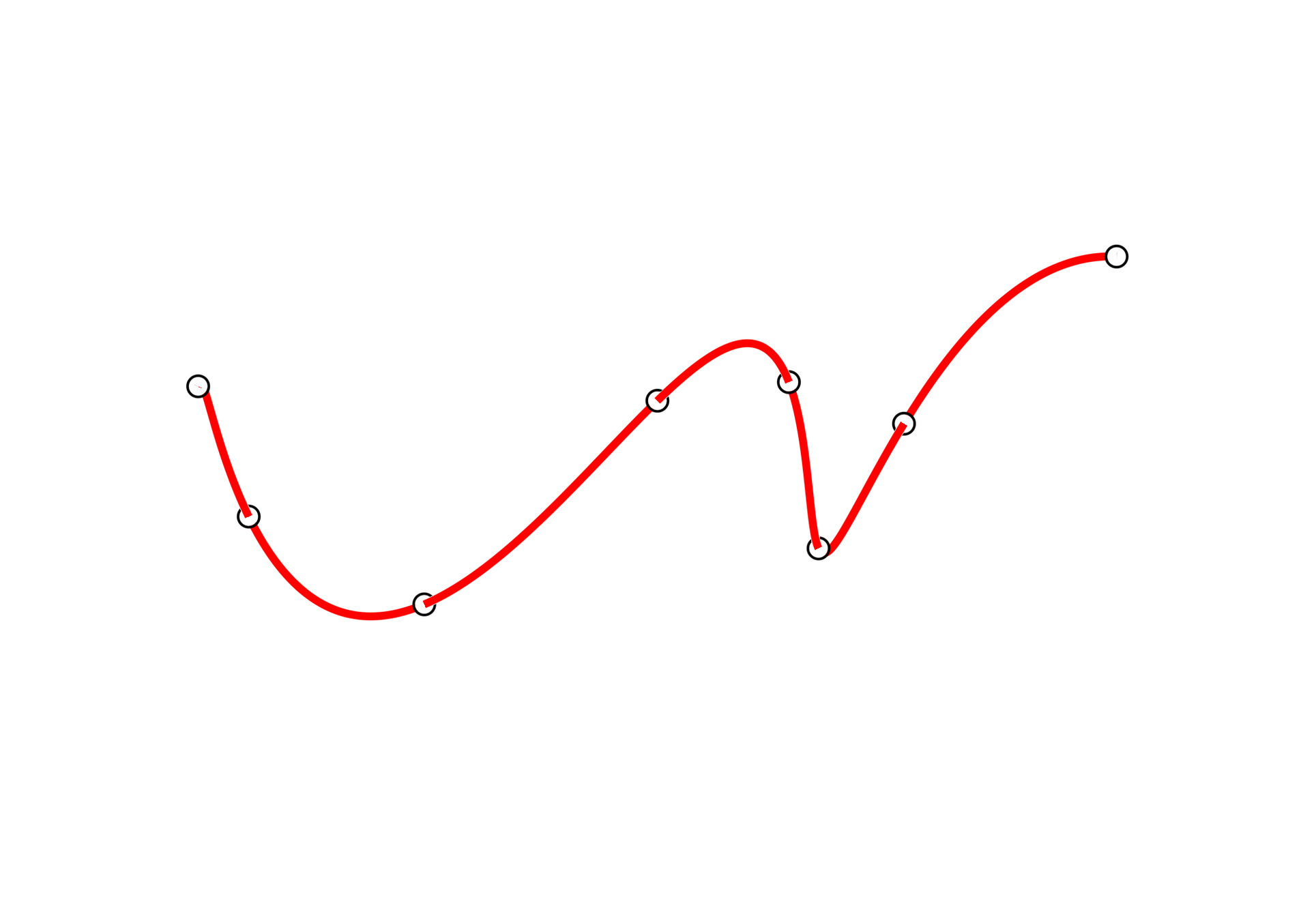
High-order interpolation is the underlying technology
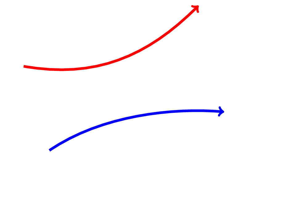
Differentiation
Interpolation
Integration
Prohibitively expensive
Challenges with meshing
Requires tailoring solution to problem
2
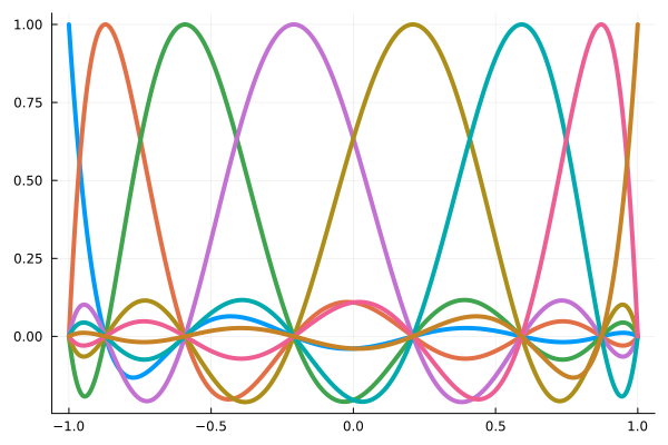
| Orthogonal Functions | Deep Neural Networks |
|---|---|
|
|
|
|
|
|
|
|
\( N \) parameters, \(M\) points
\( h \sim 1 / N \) (for shallow networks)
\( N \) points
\( \dfrac{d}{dx} \tilde{f}\sim \mathcal{O}(N^2) \) (exact)
\( \dfrac{d}{dx} \tilde{f} \sim \mathcal{O}(N) \) (exact, AD)
\( \int_\Omega \tilde{f} dx \sim \mathcal{O}(N) \) (exact)
(Weinan, 2020)
\( \int_\Omega \tilde{f} dx \sim \mathcal{O}(M) \) (approx)
Model size scales with signal complexity
Model size scales exponentially with dimension
\( N \sim h^{-d/c} \)
3
4
Landscape of ML for PDEs
Mesh ansatz
PDE-Based
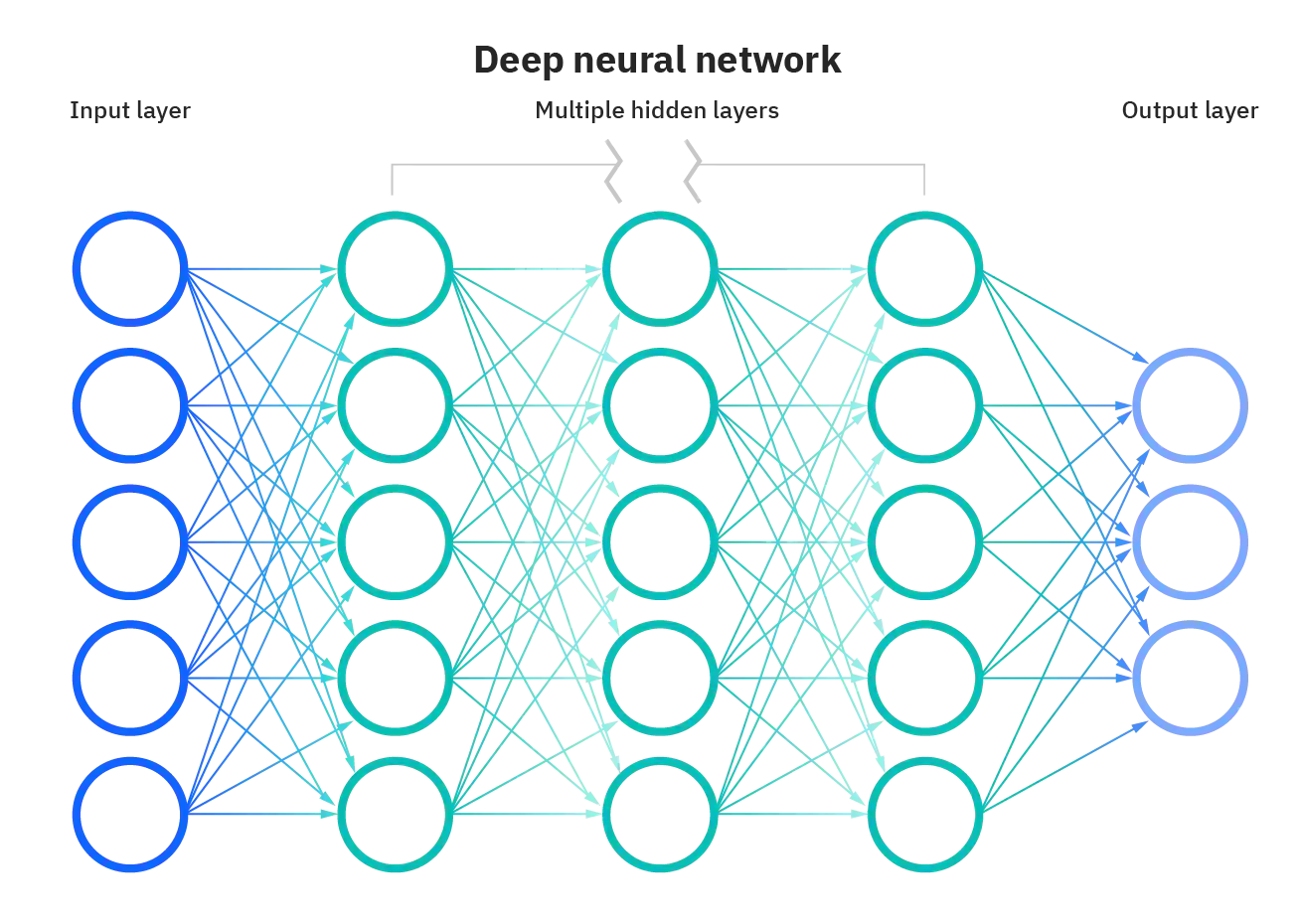
Neural Ansatz
Data-driven
FEM, FVM, IGA, Spectral
Fourier Neural Operator
Neural Field
DeepONet
Physics Informed NNs
Convolution NNs
Graph NNs
Adapted from Núñez, CEMRACS 2023
Neural ODEs
Universal Diff Eq
Reduced Order Modeling
5
1
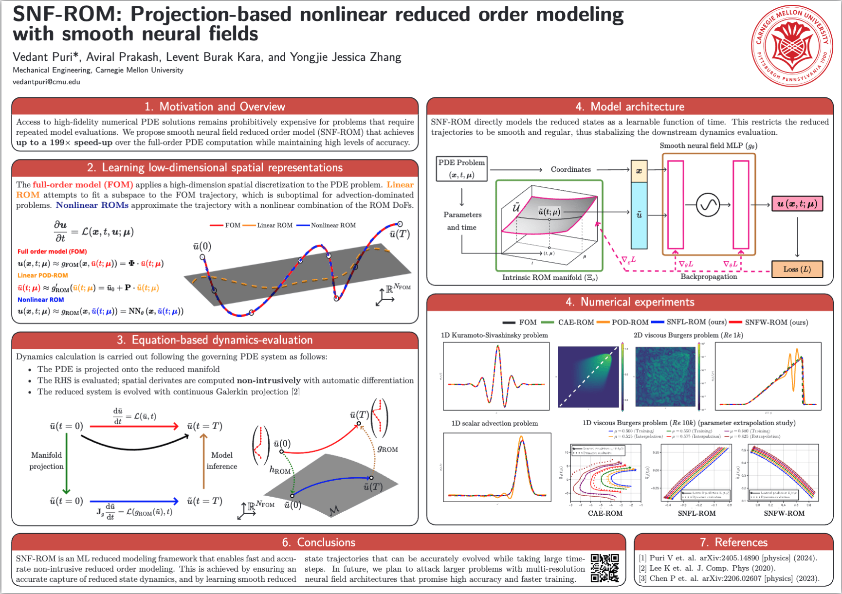
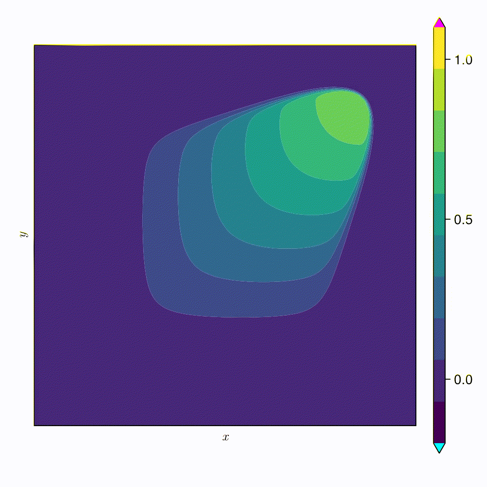
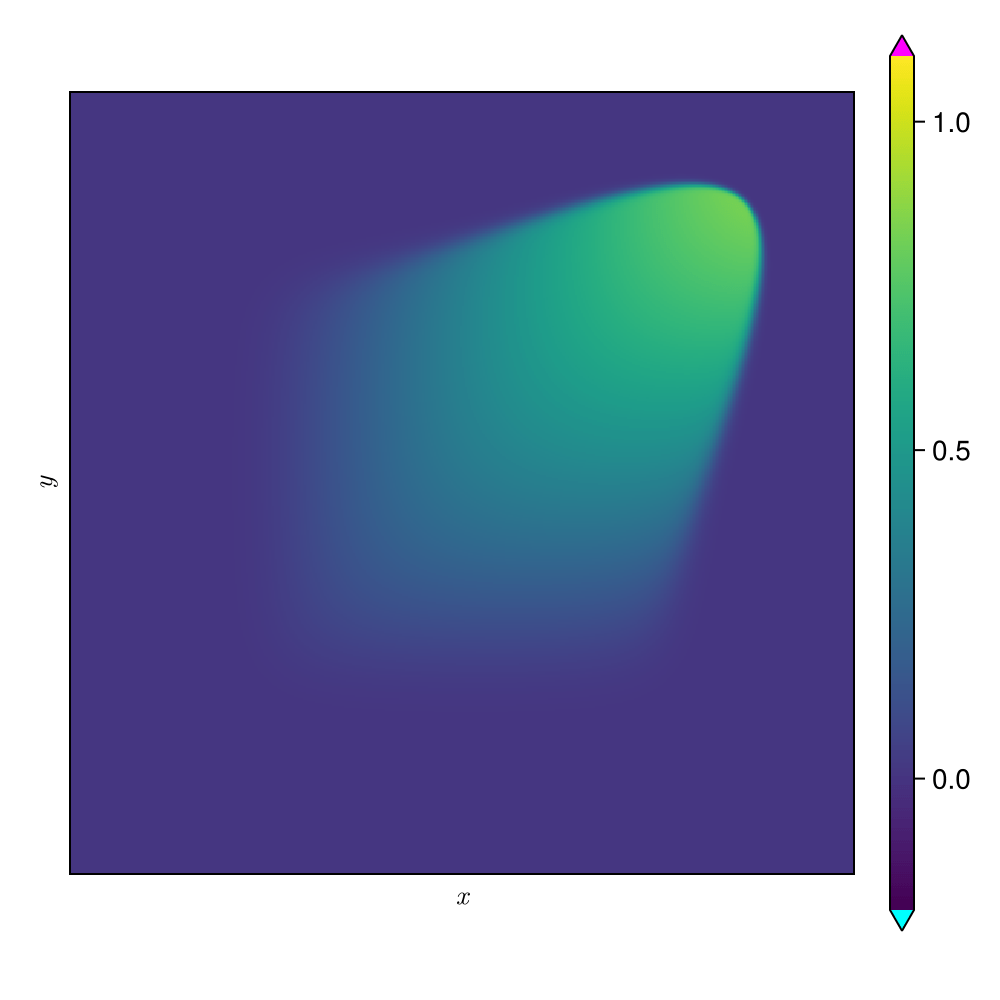
2D Viscous Burgers problem \( (\mathit{Re} = 1\text{k})\)
Smooth neural field ROM (SNF-ROM)
\(\text{Relative error: }0.37\%\)
\(\text{DoFs: }524~k \to 2\)
\(\text{Wall-time: }13.4~\text{s} \to 0.068~\text{s}\)
High freq. noise
Non-differentiable!
Accurately capture of dynamics with smooth neural fields
Large deviations!
Learning smooth latent space trajectories
\(\text{Autoencoder ROM}\)
\(\text{SNF-ROM}\)
Evolution of ROM states
No deviation
SNF-ROM ensures accurate online dynamics evaluation.
Accurate capture of dynamics
2
Full order model (FOM)
Linear POD-ROM
Nonlinear ROM
Learn low-order spatial representations
Time-evolution of reduced representation with Galerkin projection
3
Autoencoder ROMs see a sharp rise in error due to deviation of the reduced states from the learned manifold.
Encoder-free ROMs have disjoint latent space representations which inhibit online evaluations.
Autoencoder ROMs
Auto-decoder ROMs
\(\text{Encoder}\)
\(\text{Decoder}\)
\(\text{Decoder}\)
\(\text{Loss }\)
\(\nabla_{\tilde{u}} L\)
4
\(\tilde{u}(t; \boldsymbol{\mu})\)
\(\Xi_\varrho\)
Q. What prior to place on the latent space to ensure smooth/accurate traversal?
Control the complexity of latent trajectories.
Supervised learning problem: \((\boldsymbol{x}, t; \boldsymbol{\mu}) \to \boldsymbol{u}(\boldsymbol{x}, t; \boldsymbol{\mu})\).
\(\text{Loss } (L)\)
\(\text{Backpropagation}\)
\(\nabla_\theta L\)
\(\nabla_\varrho L\)
\(\nabla_\theta L\)
\(\text{PDE Problem}\)
\((\boldsymbol{x}, t, \boldsymbol{\mu})\)
\(\text{ Parameters}\)
\( \text{and time}\)
\(\text{ Intrinsic ROM manifold}\)
\(\text{Coordinates}\)
\(\text{Smooth neural field MLP }(g_\theta)\)
\(\tilde{u}\)
\(\boldsymbol{x}\)
\(\boldsymbol{u}\left( \boldsymbol{x}, t; \boldsymbol{\mu} \right)\)
Learn \((t; \boldsymbol{\mu}) \to \tilde{u}(t; \boldsymbol{\mu})\) directly
5
Derivative calculation is carried out with automatic differentiation making the dynamics evaluation non-intrusive.
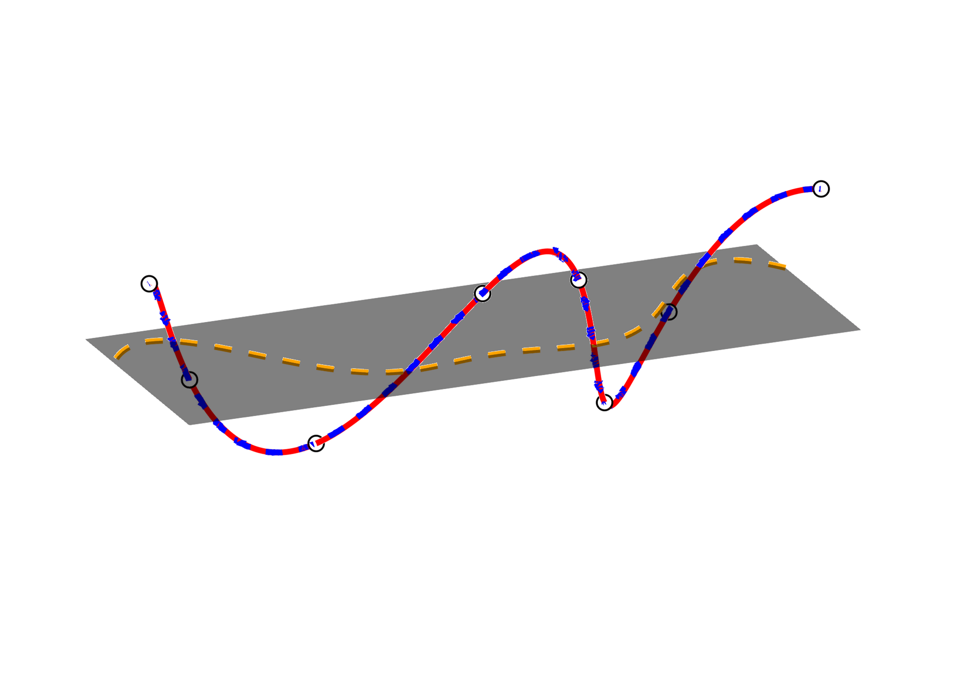
SNF-ROM with Lipschitz regularization (SNFL-ROM)
\(\text{Penalize the \textcolor{blue}{Lipschitz constant} of the MLP [arXiv:2202.08345]}\)
\(\text{[enwiki:1230354413]}\)
SNF-ROM with Weight regularization (SNFW-ROM)
\(\text{Directly penalize \textcolor{red}{high-frequency components} in }\dfrac{\text{d}}{\text{d} x}\text{NN}_\theta(x)\)
We present two approaches to learn inherently smooth and accurately differentiable neural field MLPs.
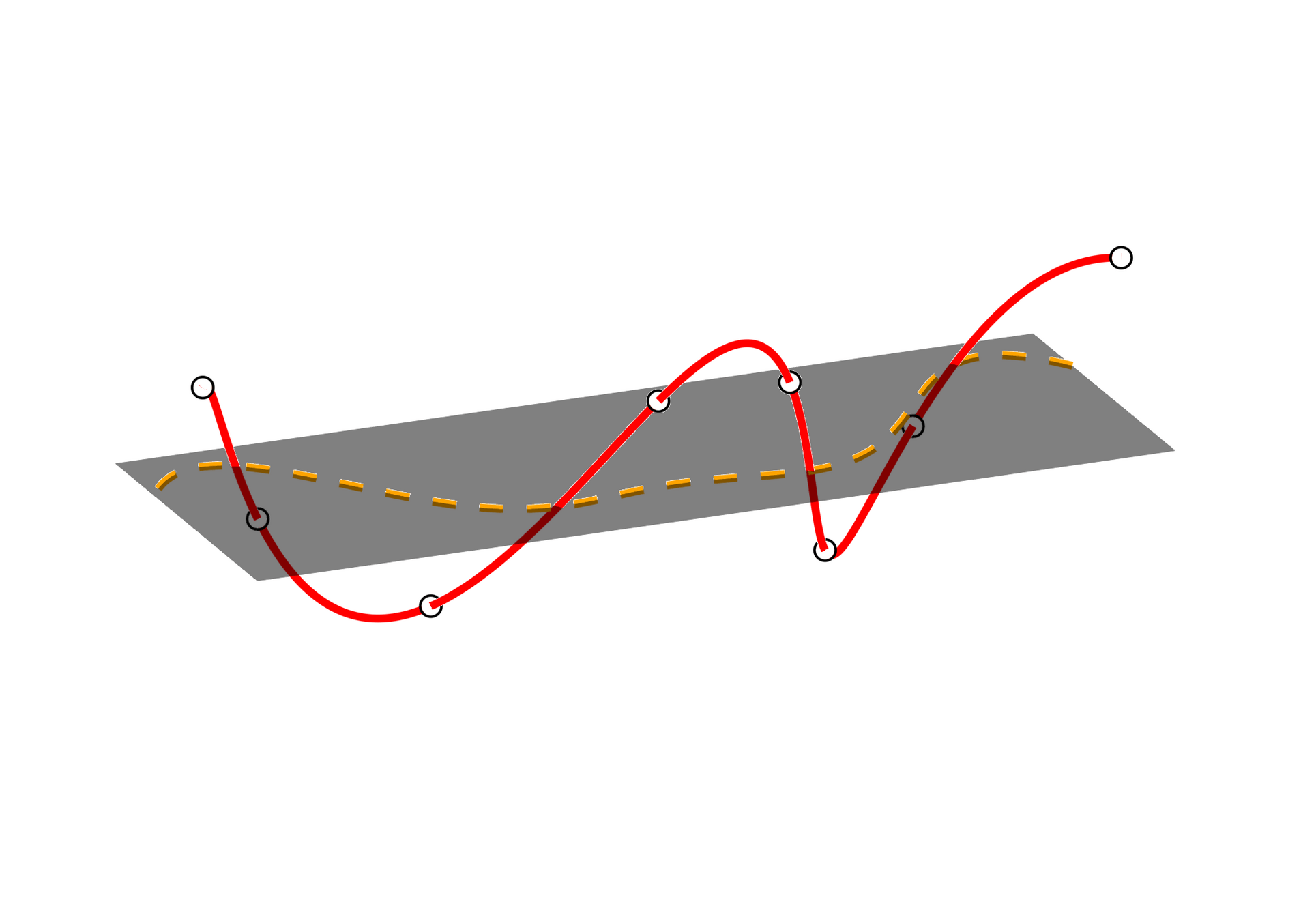
\({x}\)
\({u(x)}\)
Neural field MLPs are
non-differentiable
High freq. noise
8
Both Lipschitz regularization (SNFL) and weight regularization (SNFW) capture the 4-th order derivative accurately.
\(\text{Relative error } (\Delta t = \Delta t_0)\)
\(\text{Relative error } (\Delta t = 10\Delta t_0)\)
Oscillations due to variation in projection error
Highly diffusive; even POD with 2 modes
6
\(\text{CAE-ROM}\)
\(\text{SNFL-ROM}\)
\(\text{SNFW-ROM}\)
SNFL-ROM, SNFW-ROM effectively capture the traveling shock.
7
\(\text{CAE-ROM}\)
\(\text{SNFL-ROM}\)
\(\text{SNFW-ROM}\)
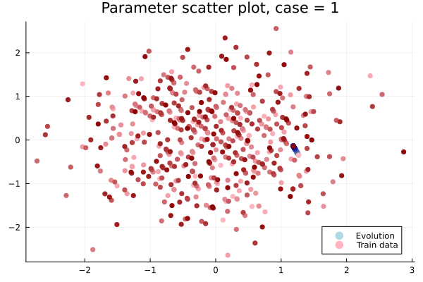
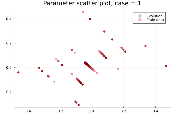
CAE-ROM has complex diverging trajectories, where as SNF-ROM has near linear and easy to follow ones
Online dynamics solve matches learned trajectories
Online evaluation deviates!
Distribution of reduced states \((\tilde{u})\)
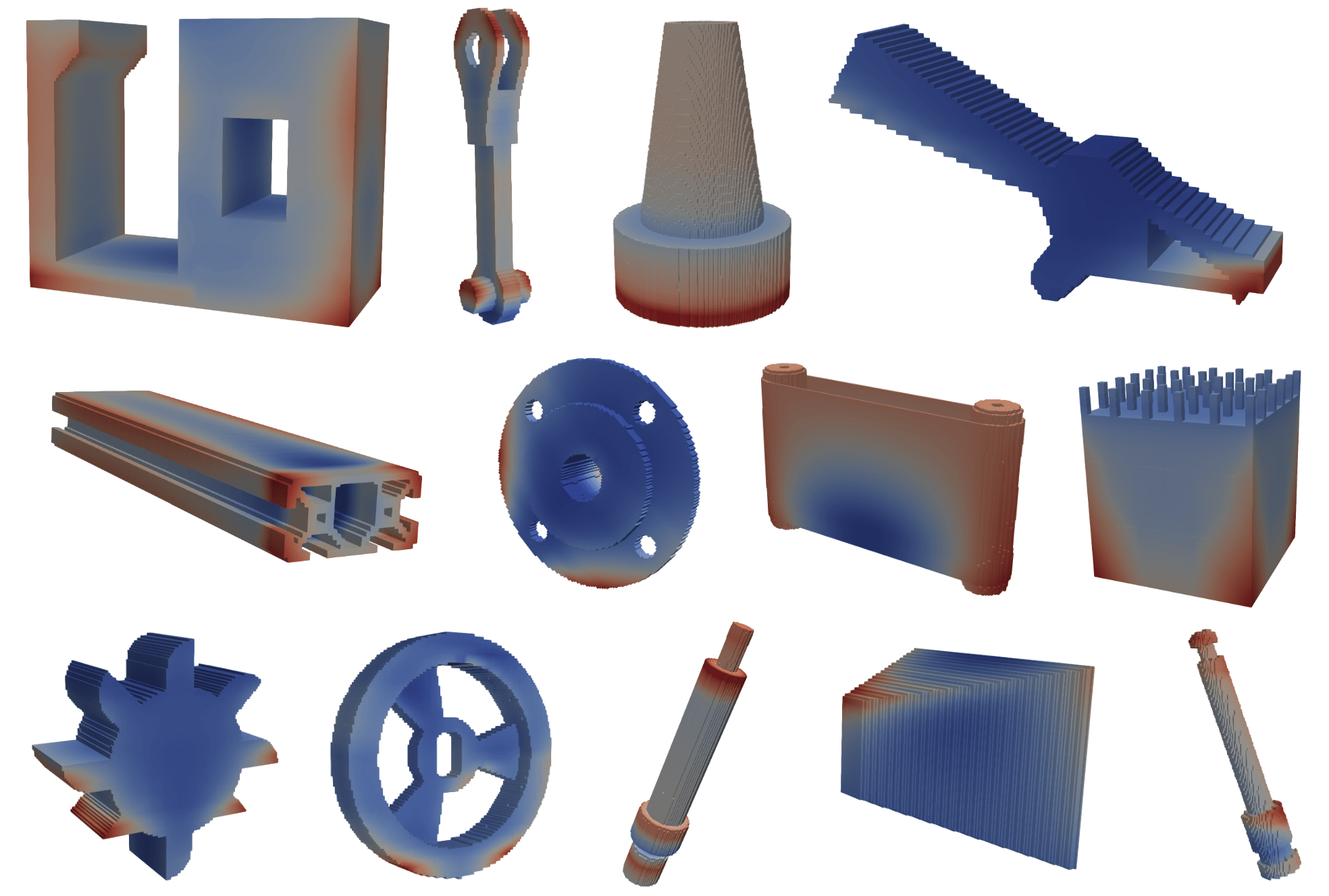
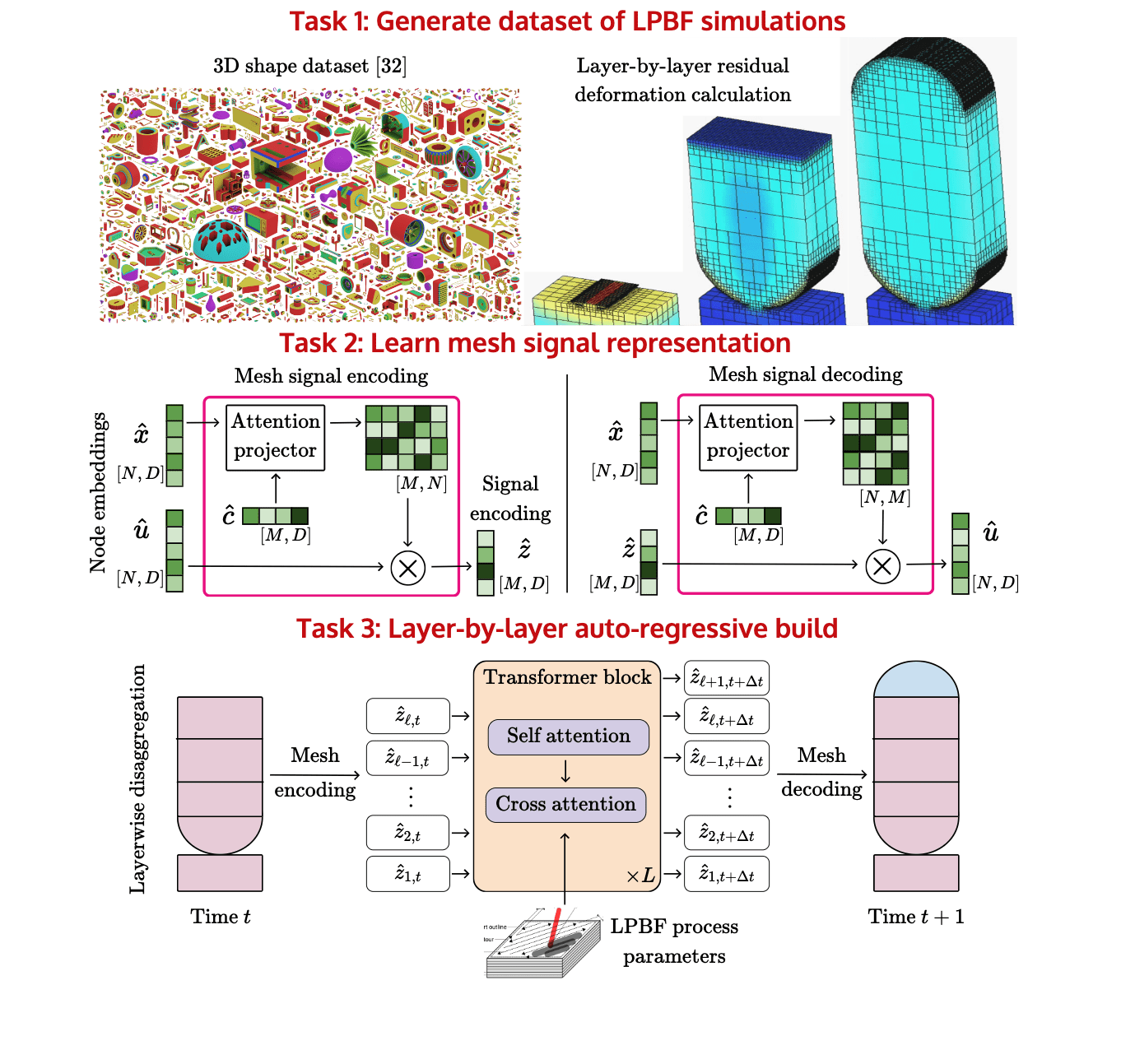
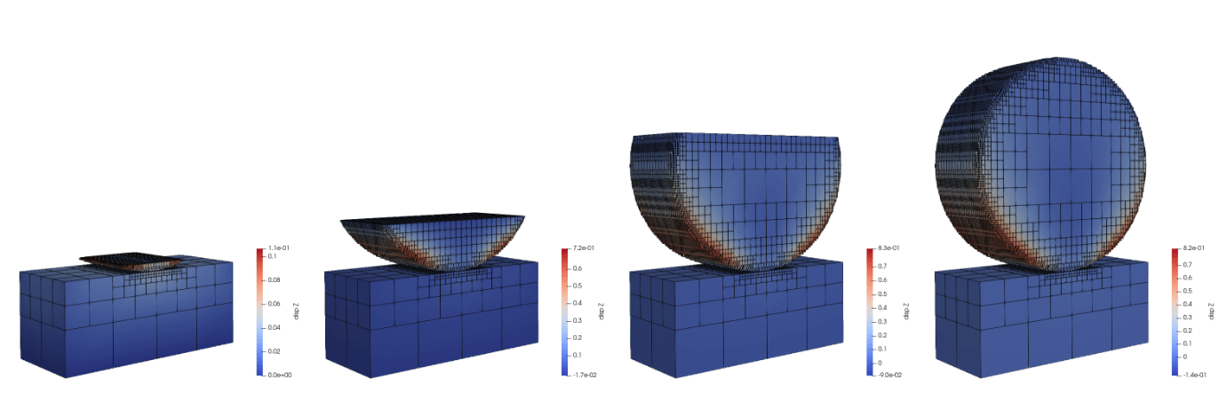
Dataset of additive manufacturing parts
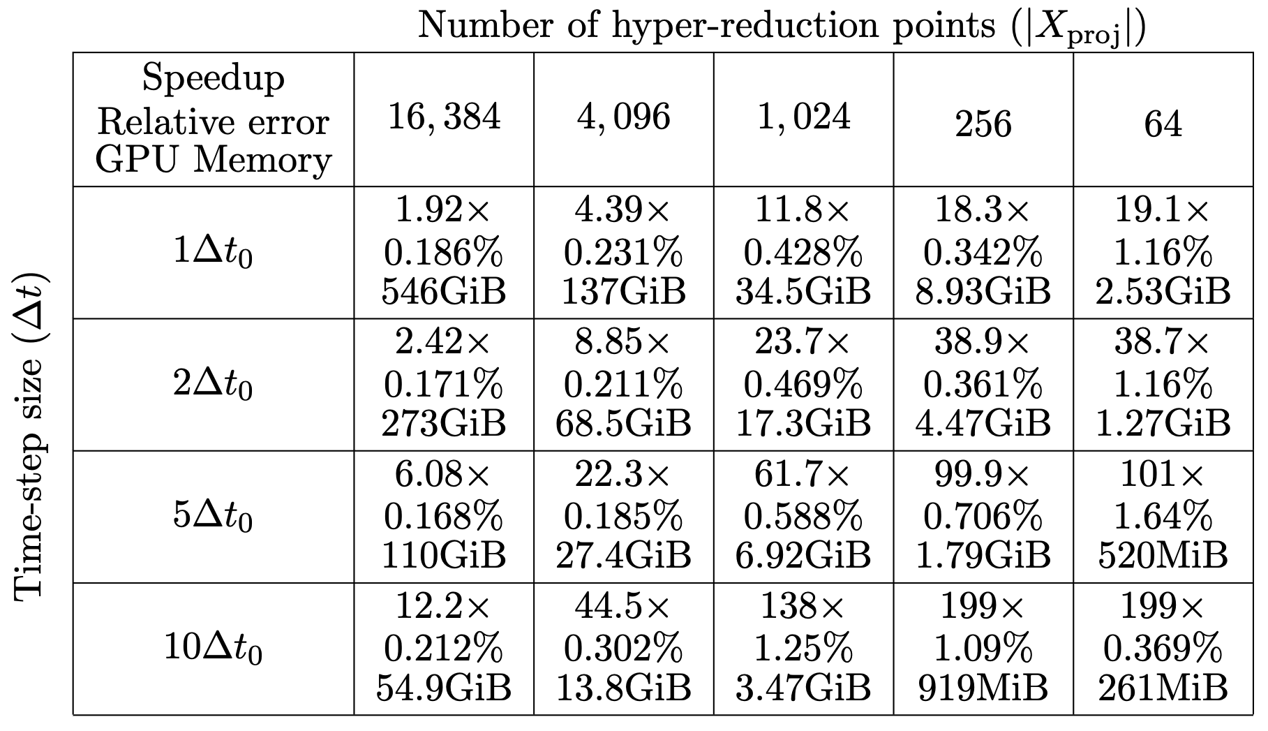
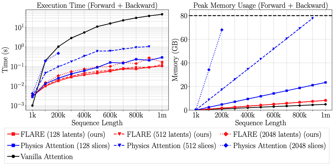
Scale up to 1 million points on a single GPU!
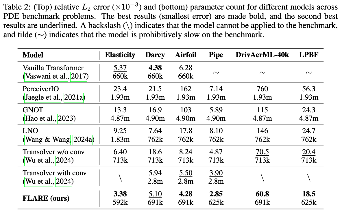
State of the art results on several PDE benchmarks!
Relative \(L_2\) error
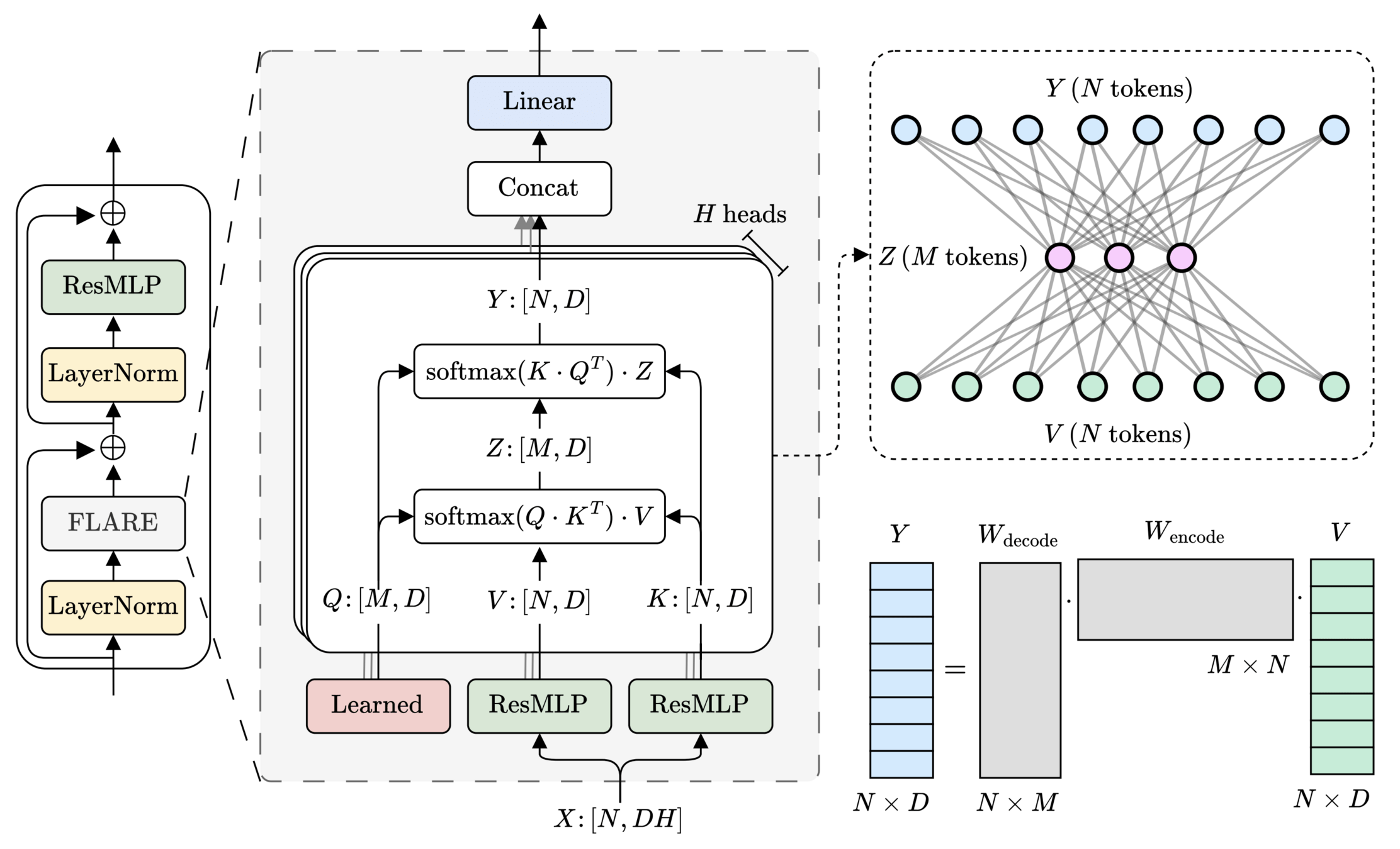
Message-passing is fundamentally low-rank
import torch.nn.functional as F
def flare_multihead_mixer(q, k, v):
	# Args - q: [H, M, D], k, v: [B, H, N, D]
	# Ret - y: [B, H, N, D]
	z = F.scaled_dot_product_attention(q, k, v, scale=1.0)
	y = F.scaled_dot_product_attention(k, q, z, scale=1.0)
return yMessage-passing is fundamentally low-rank
Continued improvement with depth and rank.
Elasticity problem
Darcy problem
1
1
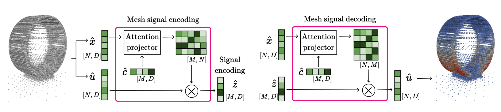
The challenge is geometry tokenization!
1
We learn an attention-based encoding scheme for tokenizing unstructured data that can be deployed on arbitrary point clouds
1
By Vedant Puri
Summary deck


