learning curves

of kernel methods

• Learn from examples: how many are needed?
  
  
   
• We consider regression (fitting functions)
  
  
   
• We study (synthetic) Gaussian random data and real data

  supervised deep learning

• Performance is evaluated through the generalization error \(\epsilon\)
  
  
   
• Learning curves decay with number of examples \(n\), often as
  
  
   
• \(\beta\) depends on the dataset and on the algorithm
   

Deep networks: \(\beta\sim 0.07\)-\(0.35\) [Hestness et al. 2017]

  learning curves

\(\epsilon\sim n^{-\beta}\)

We lack a theory for \(\beta\) for deep networks!

• Performance increases with overparametrization
  
  
    \(\longrightarrow\) study the infinite-width limit!
  
  
  
  
  
   

  link with kernel learning

\(h\)

[Neyshabur et al. 2017, 2018, Advani and Saxe 2017]

[Spigler et al. 2018, Geiger et al. 2019, Belkin et al. 2019]

\(h\)

• With a specific scaling, infinite-width limit \(\to\) kernel learning

[Rotskoff and Vanden-Eijnden 2018, Mei et al. 2017, Jacot et al. 2018, Chizat and Bach 2018, ...] 

• Very brief introduction to kernel methods and real data
  
  
   

• Gaussian data: Teacher-Student regression
  
  
   
• Smoothness of Gaussian data
  
  
   
• Effective dimension and effective smoothness in real data

  outline

• Kernel methods learn non-linear functions
   
• Map data to a feature space, where the problem is linear

data \(\underline{x} \longrightarrow \underline{\phi}(\underline{x}) \longrightarrow \) use linear combination of features

\(\underline{\phi}(\underline{x})\)

  kernel methods

• Target function  \(\underline{x}_\mu \to Z(\underline{x}_\mu),\ \ \mu=1,\dots,n\)
  
  
   
• Build an estimator  \(\hat{Z}_K(\underline{x}) = \sum_{\mu=1}^n c_\mu K(\underline{x}_\mu,\underline{x})\)
  
  
   
• Minimize training MSE \(= \frac1n \sum_{\mu=1}^n \left[ \hat{Z}_K(\underline{x}_\mu) - Z(\underline{x}_\mu) \right]^2\)
  
  
   
• Estimate the generalization error \(\epsilon = \mathbb{E}_{\underline{x}} \left[ \hat{Z}_K(\underline{x}) - Z(\underline{x}) \right]^2\)

  kernel regression

Regression: performance depends on the target function!


 

• With the weakest hypotheses, \(\beta=\frac1d\)
  
  
  
   

• With strong smoothness assumptions, \(\beta\geq\frac12\) is independent of \(d\)

  previous works

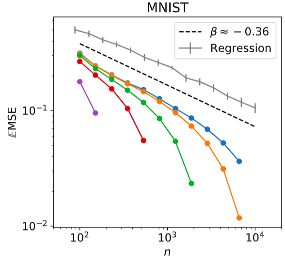
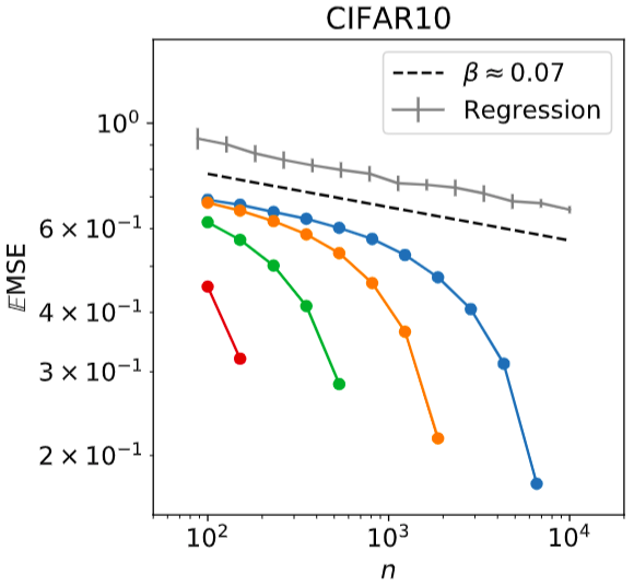
  real data

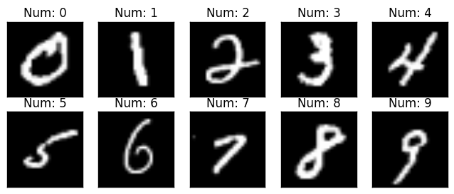
MNIST

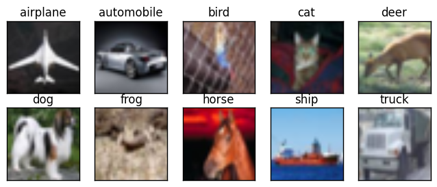
CIFAR10

2 classes: even/odd

70000 28x28 b/w pictures

2 classes: first 5/last 5

60000 32x32 RGB pictures

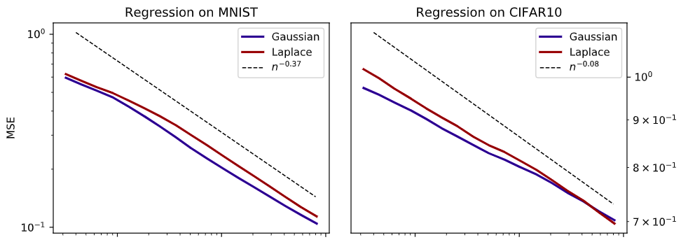
Kernel regression on:

dimension \(d = 784\)

dimension \(d = 3072\)

• Same exponent for Gaussian and Laplace kernel
  
   
• MNIST and CIFAR10 display exponents \(\beta\gg\frac1d\) but \(<\frac12\)

  real data: exponents

\(\beta\approx0.37\)

\(\beta\approx0.08\)

• Controlled setting: Teacher-Student regression
  
  
   
• Training data are sampled from a Gaussian Process:
  
        \(Z_T(\underline{x}_1),\dots,Z_T(\underline{x}_n)\ \sim\ \mathcal{N}(0, K_T)\)
        \(\underline{x}_\mu\) are random on a \(d\)-dim hypersphere
  
  
   
• Regression is done with another kernel \(K_S\)

  kernel teacher-student framework

(artificial, synthetic data)

  teacher-student: simulations

Can we understand these curves?

  teacher-student: regression

where

Explicit solution:

Regression:

\(\hat{Z}_S(\underline{x}) = \sum_{\mu=1}^n c_\mu K_S(\underline{x}_\mu,\underline{x})\)

Minimize \(= \frac1n \sum_{\mu=1}^n \left[ \hat{Z}_S(\underline{x}_\mu) - Z_T(\underline{x}_\mu) \right]^2\)

  teacher-student: theorem (1/2)

To compute the generalization error:
 

• We look at the problem in the frequency domain
   
• We assume that \(\tilde{K}_S(\underline{w}) \sim |\!|\underline{w}|\!|^{-\alpha_S}\) and \(\tilde{K}_T(\underline{w}) \sim |\!|\underline{w}|\!|^{-\alpha_T}\) as\(|\!|\underline{w}|\!|\to\infty\)
  
  
  
   
• SIMPLIFYING ASSUMPTION: We take the \(n\) points \(\underline{x}_\mu\) on a regular \(d\)-dim lattice!

  teacher-student: theorem (2/2)

• Large \(\alpha \rightarrow\) fast decay at high freq \(\rightarrow\) indifference to local details
  
   
• \(\alpha_T\) is intrinsic to the data (T), \(\alpha_S\) depends on the algorithm (S)
  
   
• If \(\alpha_S\) is large enough, \(\beta\)  takes the largest possible value \(\frac{\alpha_T - d}{d}\)
  
   
• As soon as \(\alpha_S\) is small enough, \(\beta=\frac{2\alpha_S}d\)

(optimal learning)

• If Teacher=Student=Laplace
  
  
  
  
   
• If Teacher=Gaussian, Student=Laplace

What is the prediction for our simulations?

(curse of dimensionality!)

(\(\alpha_T=\alpha_S=d+1\))

(\(\alpha_T=\infty, \alpha_S=d+1\))

  teacher-student: comparison (1/2)

• Our result matches the numerical simulations
   
• There are finite size effects (small \(n\))

(on hypersphere)

  TEACHER-STUDENT: COMPARISON (2/2)

Same result with points on regular lattice or random hypersphere?

What matters is how nearest-neighbor distance \(\delta\) scales with \(n\)

  nearest-neighbor distance

In both cases  \(\delta\sim n^{\frac1d}\)

Finite size effects: asymptotic scaling only when \(n\) is large enough

(conjecture)

  smoothness

• For Gaussian data, \(\alpha_T-d \equiv 2s\) is a measure of smoothness \(\sim\) # of continuous derivatives
  
  
  
  
  
  
  
   
• Can we say something about real data?

  what about real data?

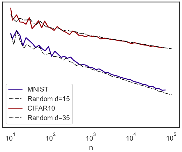
​1. Effective dimension is much smaller:

\(\delta\sim n^{\frac1{d_\mathrm{eff}}}\)

2. We find the same exponent regardless of the student:

Assuming this formula holds

  kernel pca

• \(\mathbb{K}_S\) is the Gram matrix,    \(\lambda_1\geq\lambda_2\geq\dots\) are its eigenvalues,
  \((\underline{\phi}_\rho)_{\rho\geq1}\) are its eigenvectors
  
   
• Given a Teacher Gaussian process \(\underline{Z}_T\), we can project it on this basis to compute
  
  
   
• \(q_\rho\) is a Gaussian variable, with
   

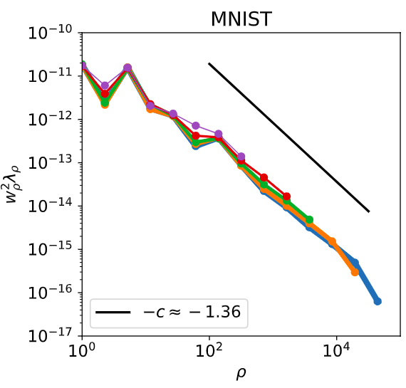
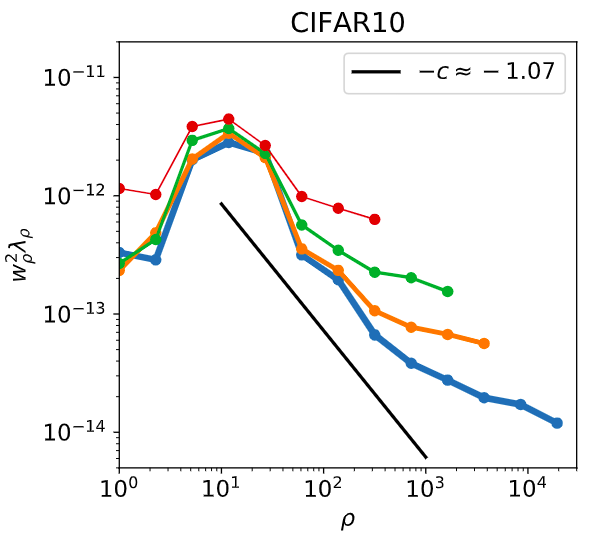
  projection of real data

Measure effective smoothness in real data

Fit \(c=\frac{\alpha_T}d\) from the projection

  exponent of real data (1/3)

  exponent of real data (2/3)

  exponent of real data (3/3)

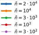
eigenmodes are extracted from a Gram matrix with a larger training set of size \(\tilde{n}\)

  conclusion

• Learning curves of real data decay as power laws with exponents
  
  
  
   
• We justify how different kernels can lead to the same exponent \(\beta\)
  
   
• We link \(\beta\) to the smoothness and dimension of the Gaussian data
  
   
• Real data live in manifolds of small effective dimension and we can define an effective smoothness that correlates with \(\beta\)
  
   
• Open question: what fixes the smoothness in real data?

arXiv:1905.10843