Spectrum Dependent Learning Curves in Kernel Regression and Wide Neural Networks

Overview

Setting: kernel regression for a generic target function
Decompose the generalization error over the kernel's spectral components
Derive an approximate formula for the error
Validated via numerical experiments (with focus on the NTK)
Error associated with larger eigenvalues decay faster with the training size: learning through successive steps

Kernel (ridge) regression

$p$ training points $\{\mathbf x_i,f^\star(\mathbf x_i)\}_{i=1}^p$ generated by target function $f^\star:\mathbb R^d\to\mathbb R$ , $\mathbf x_i\sim p(\mathbf x_i)$
Kernel regression: $\min_{f\in\mathcal H(K)} \sum_{i=1}^p \left[ f(\mathbf x_i) - f^\star(\mathbf x_i) \right]^2 + \lambda |\!|f|\!|_K$
Estimator: $f(\mathbf x) = \mathbf y^t (\mathbb K + \lambda\mathbb I)^{-1} \mathbf k(\mathbf x)$
Generalization error:

$y_i = f^\star(\mathbf x_i)$

$\mathbb K_{ij} = K(\mathbf x_i,\mathbf x_j)$

$k_i(\mathbf x) = K(\mathbf x,\mathbf x_i)$

E_g = \left\langle \int\mathrm d^d\mathbf x p(\mathbf x) \left[f(\mathbf x) - f^\star(\mathbf x)\right]^2 \right\rangle_{\{\mathbf x_i\}, f^\star}

E_g = \left\langle \int\mathrm d^d\mathbf x p(\mathbf x) \left[f(\mathbf x) - f^\star(\mathbf x)\right]^2 \right\rangle_{\{\mathbf x_i\}, f^\star}

Mercer decomposition

K(\mathbf x,\mathbf x^\prime) = \sum_{\rho=1}^\textcolor{red}{M} \lambda_\rho \phi_\rho(\mathbf x) \phi_\rho(\mathbf x^\prime) \equiv \sum_{\rho=1}^\textcolor{red}{M} \psi_\rho(\mathbf x) \psi_\rho(\mathbf x^\prime)

\int \mathrm d^d\mathbf x^\prime p(\mathbf x^\prime) K(\mathbf x,\mathbf x^\prime) \phi_\rho(\mathbf x^\prime) = \lambda_\rho \phi_\rho(\mathbf x)

\int \mathrm d^d\mathbf x^\prime p(\mathbf x^\prime) K(\mathbf x,\mathbf x^\prime) \phi_\rho(\mathbf x^\prime) = \lambda_\rho \phi_\rho(\mathbf x)

$\{\lambda_\rho,\phi_\rho\}$ are the kernel's eigenstates
$\{\phi_\rho\}$ are chosen to form an orthonormal basis:

\left\langle \phi_\rho(\mathbf x) \phi_\gamma(\mathbf x)\right\rangle_{\mathbf x} = \int \mathrm d^d\mathbf x p(\mathbf x) \phi_\rho(\mathbf x) \phi_\gamma(\mathbf x) = \delta_{\rho\gamma}

\left\langle \phi_\rho(\mathbf x) \phi_\gamma(\mathbf x)\right\rangle_{\mathbf x} = \int \mathrm d^d\mathbf x p(\mathbf x) \phi_\rho(\mathbf x) \phi_\gamma(\mathbf x) = \delta_{\rho\gamma}

Kernel regression in feature space

Expand the target and estimator functions in the kernel's basis:

$f^\star(\mathbf x) = \sum_\rho \bar w_\rho \psi_\rho(\mathbf x)$
$f(\mathbf x) = \sum_\rho w_\rho \psi_\rho(\mathbf x)$
Then kernel regression can be written as

$\min_{\mathbf w,\ |\!|\mathbf w|\!|<\infty} |\!|\Psi^t \mathbf w - \mathbf y|\!|^2 + \lambda |\!|\mathbf w|\!|^2$
And its solution is $\mathbf w = \left(\Psi\Psi^t + \lambda\mathbb I\right)^{-1} \Psi \mathbf y$

design matrix $\Psi_{\rho,i}=\psi_\rho(\mathbf x_i)$

e.g. Teacher = Gaussian:

f^\star(\mathbf x) = \sum_\rho \bar w^T_\rho \psi^T_\rho(\mathbf x)

f^\star(\mathbf x) = \sum_\rho \bar w^T_\rho \psi^T_\rho(\mathbf x)

\bar w_\rho = \bar w^T_\rho \sqrt{\frac{\lambda^T_\rho}{\lambda_\rho}}

\bar w_\rho = \bar w^T_\rho \sqrt{\frac{\lambda^T_\rho}{\lambda_\rho}}

\bar\mathbf w^T \sim \mathcal N(0,\mathbb I)

Generalization error and spectral components

We can then derive $E_g = \sum_\rho E_\rho$ , with

where

E_\rho = \lambda_\rho \left\langle (w_\rho - \bar w_\rho)^2 \right\rangle_{\{\mathbf x_i\}, \bar\mathbf w_\rho} = \sum_\gamma \mathbf D_{\rho\gamma} \left\langle \mathbf G^2_{\gamma\rho} \right\rangle_{\{\mathbf x_i\}}

\mathbf D = \Lambda^{-\frac12} \left\langle \bar\mathbf w \bar\mathbf w^t\right\rangle_{\bar\mathbf w} \Lambda^{-\frac12}

\mathbf G = \left( \frac1\lambda \Phi\Phi^t + \Lambda^{-1} \right)^{-1}

\mathbf G = \left( \frac1\lambda \Phi\Phi^t + \Lambda^{-1} \right)^{-1}

\Phi = \Lambda^{-\frac12} \Psi

\Phi = \Lambda^{-\frac12} \Psi

\Lambda_{\rho\gamma} = \lambda_\rho \delta_{\rho\gamma}

\Lambda_{\rho\gamma} = \lambda_\rho \delta_{\rho\gamma}

the target function is only here!

the data points are only here!

Approximation for $\left\langle G^2 \right\rangle$

$\tilde\mathbf G(p,v) \equiv \left( \frac1\lambda \Phi\Phi^t + \Lambda^{-1} + v\mathbb I \right)^{-1}$
Derive a recurrence equation for the addition of a $p+1$ -st point, $\mathbf x_{p+1}$ corresponding to $\mathbf \phi = (\phi_\rho(\mathbf x_{p+1}))_\rho$ :
Use Sherman-Morrison formula (Woodbury inversion)

\tilde\mathbf G (p,0) = \mathbf G, \quad \left\langle \mathbf G^2 \right\rangle = -\partial_v \left\langle \tilde\mathbf G(p,v) \right\rangle_{v=0}

\left\langle \tilde\mathbf G(p + 1,v) \right\rangle_{\{\mathbf x_i\}_{i=1}^{p+1}} = \left\langle \left(\tilde\mathbf G(p,v)^{-1} + \frac1\lambda \mathbf\phi \mathbf\phi^t\right)^{-1} \right\rangle_{\{\mathbf x_i\}_{i=1}^{p+1}}

(A + \mathbf v \mathbf v^t)^{-1} = A^{-1} - \frac{A^{-1} \mathbf v \mathbf v^t A^{-1}}{1 + \mathbf v^t A^{-1} \mathbf v}

(A + \mathbf v \mathbf v^t)^{-1} = A^{-1} - \frac{A^{-1} \mathbf v \mathbf v^t A^{-1}}{1 + \mathbf v^t A^{-1} \mathbf v}

Approximation for $\left\langle G^2 \right\rangle$

First approximation: approximate the second term as
Second approximation: continuous $p \to$ PDE

\left\langle \tilde\mathbf G(p + 1,v) \right\rangle_{\{\mathbf x_i\}_{i=1}^{p+1}} = \left\langle \tilde\mathbf G(p,v) \right\rangle_{\{\mathbf x_i\}_{i=1}^{\textcolor{red}{p}}} - \left\langle \frac{ \tilde\mathbf G(p,v) \mathbf\phi \mathbf\phi^t \tilde\mathbf G(p,v) }{ \lambda + \mathbf\phi^t \tilde\mathbf G(p,v) \mathbf\phi } \right\rangle_{\{\mathbf x_i\}_{i=1}^{p+1}}

\left\langle \tilde\mathbf G(p + 1,v) \right\rangle_{\{\mathbf x_i\}_{i=1}^{p+1}} \approx \left\langle \tilde\mathbf G(p,v) \right\rangle_{\{\mathbf x_i\}_{i=1}^{\textcolor{red}{p}}} - \frac{ \left\langle \tilde\mathbf G^2(p,v) \right\rangle_{\{\mathbf x_i\}_{i=1}^{\textcolor{red}{p}}} }{ \lambda + \mathrm{tr} \left\langle \tilde\mathbf G(p,v) \right\rangle_{\{\mathbf x_i\}_{i=1}^{\textcolor{red}{p}}} }

\partial_p \left\langle \tilde\mathbf G(p,v) \right\rangle \approx \frac1{\lambda + \mathrm{tr} \left\langle \tilde\mathbf G(p,v) \right\rangle } \partial_v \left\langle \tilde\mathbf G(p,v) \right\rangle

\tilde\mathbf G(0,v) = \left( \Lambda^{-1} + v \mathbb I \right)^{-1}

PDE solution

This linear PDE can be solved exactly (with the method of characteristics)
Then the error component $E_\rho$ is

g_\rho(p,v) \equiv \left\langle \tilde\mathbf G_{\rho\rho}(p,v) \right\rangle = \left( \frac1{\lambda_\rho} + v + \frac{p}{\lambda + \sum_\gamma g_\gamma(p,v)} \right)^{-1}

E_\rho = \frac{\left\langle \bar w_\rho^2 \right\rangle}{\lambda_\rho} \left( \frac1{\lambda_\rho} + \frac{p}{\lambda + t(p)} \right)^{-2} \left( 1 - \frac{p \gamma(p)}{\left[\lambda + t(p)\right]^2} \right)^{-1}

E_\rho = \frac{\left\langle \bar w_\rho^2 \right\rangle}{\lambda_\rho} \left( \frac1{\lambda_\rho} + \frac{p}{\lambda + t(p)} \right)^{-2} \left( 1 - \frac{p \gamma(p)}{\left[\lambda + t(p)\right]^2} \right)^{-1}

t(p) = \sum_\rho \left( \frac1{\lambda_\rho} + \frac{p}{\lambda + t(p)}\right)^{-1} \sim p^{-1}

t(p) = \sum_\rho \left( \frac1{\lambda_\rho} + \frac{p}{\lambda + t(p)}\right)^{-1} \sim p^{-1}

\gamma(p) = \sum_\rho \left( \frac1{\lambda_\rho} + \frac{p}{\lambda + t(p)}\right)^{-2} \sim p^{-2}

\gamma(p) = \sum_\rho \left( \frac1{\lambda_\rho} + \frac{p}{\lambda + t(p)}\right)^{-2} \sim p^{-2}

Note: the same result is found with replica calculations!

Comments on the result

The effect of the target function is simply a (mode-dependent) prefactor $\left\langle\bar w_\rho^2\right\rangle$
Ratio between two modes:
The error is large if the target function puts a lot of weight on small $\lambda_\rho$ modes

E_\rho = \frac{\left\langle \bar w_\rho^2 \right\rangle}{\lambda_\rho} \left( \frac1{\lambda_\rho} + \frac{p}{\lambda + t(p)} \right)^{-2} \left( 1 - \frac{p \gamma(p)}{\left[\lambda + t(p)\right]^2} \right)^{-1}

E_\rho = \frac{\left\langle \bar w_\rho^2 \right\rangle}{\lambda_\rho} \left( \frac1{\lambda_\rho} + \frac{p}{\lambda + t(p)} \right)^{-2} \left( 1 - \frac{p \gamma(p)}{\left[\lambda + t(p)\right]^2} \right)^{-1}

\frac{E_\rho}{E_\gamma} = \frac{\left\langle \bar w_\rho^2 \right\rangle}{\left\langle \bar w_\gamma^2 \right\rangle} \frac{\lambda_\gamma}{\lambda_\rho} \frac{\left( \frac1{\lambda_\gamma} + \frac{p}{\lambda + t(p)} \right)^2}{\left( \frac1{\lambda_\rho} + \frac{p}{\lambda + t(p)} \right)^2}

\frac{E_\rho}{E_\gamma} = \frac{\left\langle \bar w_\rho^2 \right\rangle}{\left\langle \bar w_\gamma^2 \right\rangle} \frac{\lambda_\gamma}{\lambda_\rho} \frac{\left( \frac1{\lambda_\gamma} + \frac{p}{\lambda + t(p)} \right)^2}{\left( \frac1{\lambda_\rho} + \frac{p}{\lambda + t(p)} \right)^2}

Small $p$ :

\frac{E_\rho}{E_\gamma} \sim \frac{\lambda_\rho \left\langle \bar w_\rho^2 \right\rangle}{\lambda_\gamma \left\langle \bar w_\gamma^2 \right\rangle} \sim \textcolor{red}{\frac{\lambda^T_\rho}{\lambda^T_\gamma}}

\frac{E_\rho}{E_\gamma} \sim \frac{\lambda_\rho \left\langle \bar w_\rho^2 \right\rangle}{\lambda_\gamma \left\langle \bar w_\gamma^2 \right\rangle} \sim \textcolor{red}{\frac{\lambda^T_\rho}{\lambda^T_\gamma}}

Large $p$ :

\frac{E_\rho}{E_\gamma} \sim \frac{\left\langle \bar w_\rho^2 \right\rangle / \lambda_\rho}{\left\langle \bar w_\gamma^2 \right\rangle / \lambda_\gamma} \sim \textcolor{red}{\frac{\lambda^T_\rho / \lambda^2_\rho}{\lambda^T_\gamma / \lambda^2_\gamma}}

\frac{E_\rho}{E_\gamma} \sim \frac{\left\langle \bar w_\rho^2 \right\rangle / \lambda_\rho}{\left\langle \bar w_\gamma^2 \right\rangle / \lambda_\gamma} \sim \textcolor{red}{\frac{\lambda^T_\rho / \lambda^2_\rho}{\lambda^T_\gamma / \lambda^2_\gamma}}

Dot-product kernels in $d\to\infty$

We consider now $K(\mathbf x,\mathbf x^\prime) = K(\mathbf x\cdot\mathbf x^\prime)$ , $\mathbf x\in\mathbb S^{d-1}$
Eigenstates are spherical harmonics, eigenvalues are degenerate:

e.g. NTK

(everything I say next could be derived for translation-invariant kernels as well)

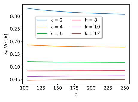
K(\mathbf x\cdot\mathbf x^\prime) = \sum_{k\geq0} \lambda_k \sum_{m=1}^{N(d,k)} Y_{km}(\mathbf x) Y_{km}(\mathbf x^\prime)

K(\mathbf x\cdot\mathbf x^\prime) = \sum_{k\geq0} \lambda_k \sum_{m=1}^{N(d,k)} Y_{km}(\mathbf x) Y_{km}(\mathbf x^\prime)

for $d\to\infty$ , $N(d,k)\sim d^k$

and $\lambda_k \sim N(d,k)^{-1} \sim d^{-k}$

NTK

Dot-product kernels in $d\to\infty$

Learning proceeds by stages. Take $p = \alpha d^\ell$ :
Modes with larger $\lambda_k$ are learned earlier!

\frac{E_{km}(\alpha)}{E_{km}(0)} =

\frac{E_{km}(\alpha)}{E_{km}(0)} =

0, \quad\mathrm{for}\, k < \ell

0, \quad\mathrm{for}\, k < \ell

1, \quad\mathrm{for}\, k > \ell

1, \quad\mathrm{for}\, k > \ell

\frac{\mathrm{const}}{\alpha^2}, \quad\mathrm{for}\, k = \ell

\frac{\mathrm{const}}{\alpha^2}, \quad\mathrm{for}\, k = \ell

\underbrace{\phantom{wwwwwwww}}

\underbrace{\phantom{wwwwwwww}}

Numerical experiments

Three settings are considered:

Kernel Teacher-Student with 4-layer NTK kernels (for both)
Finite-width NNs learning pure modes
Finite-width Teacher-Student 2-layer NNs

f^\star(\mathbf x) = \sum_{i=1}^{p^\prime} \bar\alpha_i K^{\mathrm{NTK}}(\mathbf x\cdot\mathbf x_i) \ \to

f^\star(\mathbf x) = \sum_{i=1}^{p^\prime} \bar\alpha_i K^{\mathrm{NTK}}(\mathbf x\cdot\mathbf x_i) \ \to

kernel regression with $K^\mathrm{NTK}$

f^\star(\mathbf x) = \sum_{i=1}^{p^\prime} \bar\alpha_i \sum_{m=1}^{N(d,k)} Y_{km}(\mathbf x)Y_{km}(\mathbf x_i) \equiv \sum_{i=1}^{p^\prime} \bar\alpha_i Q_k(\mathbf x\cdot\mathbf x_i)

f^\star(\mathbf x) = \sum_{i=1}^{p^\prime} \bar\alpha_i \sum_{m=1}^{N(d,k)} Y_{km}(\mathbf x)Y_{km}(\mathbf x_i) \equiv \sum_{i=1}^{p^\prime} \bar\alpha_i Q_k(\mathbf x\cdot\mathbf x_i)

$\to$ learn with NNs (4 layers h=500, 2 layers h=10000)

f^\star(\mathbf x) = \bar\mathbf r \cdot \sigma(\bar\mathbf\Theta \mathbf x) \to \ \mathrm{learn\ with} \ f(\mathbf x) = \mathbf r \cdot \sigma(\mathbf\Theta \mathbf x)

Note: this contains several spherical harmonics

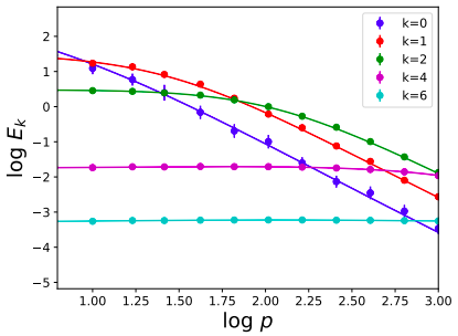
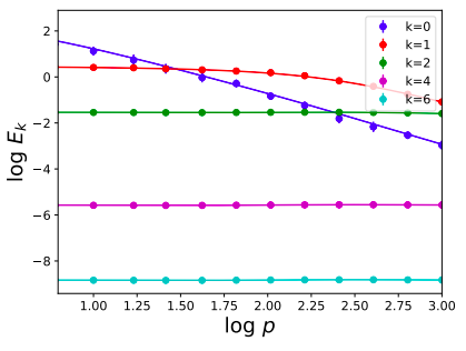
Kernel regression with 4-layer NTK kernel

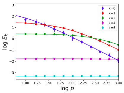
$d=10,\ \lambda=5$

$d=10,\ \lambda=0$ ridgeless

$d=100,\ \lambda=0$ ridgeless

$E_k = \sum_{m=1}^{N(d,k)} E_{km} = N(d,k) E_{k,1}$

Pure $\lambda_k$ modes with NNs

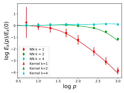
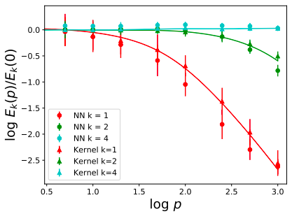
2 layers, width 10000

4 layers, width 500

f^\star(\mathbf x) = \sum_{i=1}^{p^\prime} \bar\alpha_i \sum_{m=1}^{N(d,\textcolor{red}{k})} Y_{\textcolor{red}{k}m}(\mathbf x)Y_{\textcolor{red}{k}m}(\mathbf x_i) \equiv \sum_{i=1}^{p^\prime} \bar\alpha_i Q_\textcolor{red}{k}(\mathbf x\cdot\mathbf x_i)

$f^\star$ has only the $\textcolor{red}{k}$ mode

$d=30$

Teacher-Student 2-layer NNs

f^\star(\mathbf x) = \bar\mathbf r \cdot \sigma(\bar\mathbf\Theta \mathbf x) \to \ \mathrm{learn\ with} \ f(\mathbf x) = \mathbf r \cdot \sigma(\mathbf\Theta \mathbf x)

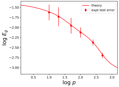
$d=25$ , width 8000

Spectrum Dependent Learning Curves in Kernel Regression

Journal club

Spectrum Dependent Learning Curves in Kernel Regression and Wide Neural Networks

Spectrum Dependent Learning Curves in Kernel Regression and Wide Neural Networks

Stefano Spigler

Spectrum Dependent Learning Curves in Kernel Regression

Journal club

Spectrum Dependent Learning Curves in Kernel Regression and Wide Neural Networks

More from Stefano Spigler