Loss Landscape and

Performance in Deep Learning

M. Geiger, A. Jacot, S. d’Ascoli, M. Baity-Jesi,

L. Sagun, G. Biroli, C. Hongler, M. Wyart

Stefano Spigler

arXivs: 1901.01608; 1810.09665; 1809.09349

(Supervised) Deep Learning

$<-1$

$>+1$

Learning from examples: train set
Is able to predict: test set
Not understood why it works so well!

$f(\mathbf{x})$

How many data are needed to learn?
What network size?

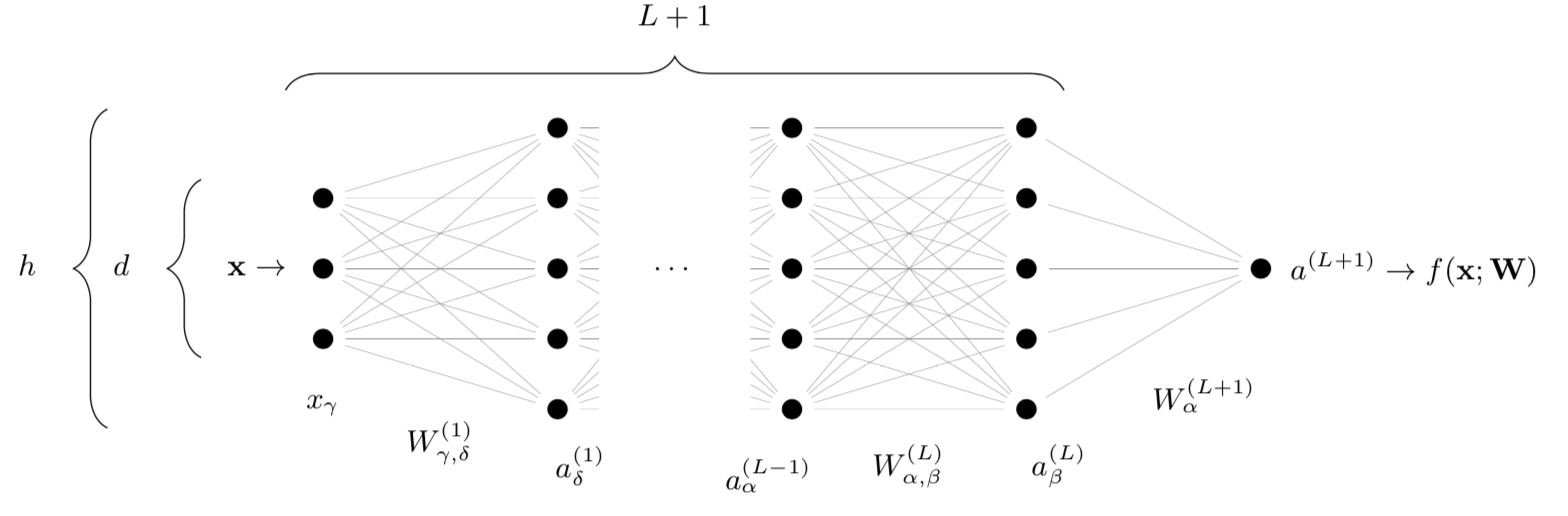
Set-up: Architecture

Deep net $f(\mathbf{x};\mathbf{W})$ with $\textcolor{red}{N}\sim h^2L$ parameters

depth $L$

width $\color{red}h$

$f(\mathbf{x};\mathbf{W})$

Alternating linear and nonlinear operations!

$W_\mu$

Set-up: Dataset

$\color{red}P$ training data:
$\mathbf{x}_1, \dots, \mathbf{x}_P$
Binary classification:
$\mathbf{x}_i \to \mathrm{label}\ y_i = \pm1$
Independent test set to evaluate performance

Example - MNIST (parity):

70k pictures, digits $0,\dots,9$;

use parity as label

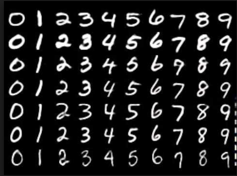
$\pm1=$ cats/dogs, yes/no, even/odd...

Outline

Vary network size $\color{red}N$ ($\sim\color{red}h^2$):

Can networks fit all the $\color{red}P$ training data?
Can networks overfit? Can $\color{red}N$ be too large?

$\to$ Long term goal: how to choose $\color{red}N$?

$h$

Learning

Find parameters $\mathbf{W}$ such that $\mathrm{sign} f(\mathbf{x}_i; \mathbf{W}) = y_i$ for $i\in$ train set
Minimize some loss!
$\mathcal{L}(\mathbf{W}) = 0$ if and only if $y_i f(\mathbf{x}_i;\mathbf{W}) > 1$ for all patterns

\displaystyle \mathcal{L}(\mathbf{W}) = \sum_{i=1}^P {\color{red}\ell\left( {\color{black}y_i f(\mathbf{x}_i;\mathbf{W})} \right)}

(classified correctly with some margin)

Binary classification: $y_i = \pm1$

Hinge loss:

Learning dynamics = descent in loss landscape

Minimize loss $\longleftrightarrow$ gradient descent
Start with random initial conditions!

Random, high dimensional, not convex landscape!

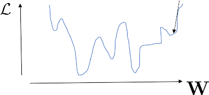
Why not stuck in bad local minima?
What is the landscape geometry?
Many flat directions are found!

bad local minimum?

Soudry, Hoffer '17; Sagun et al. '17; Cooper '18; Baity-Jesy et al. '18 - arXiv:1803.06969

in practical settings:

Analogy with granular matter: Jamming

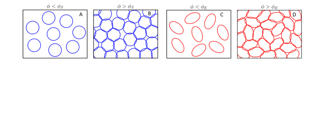
Upon increasing density $\to$ transition

sharp transition with finite-range interactions

random initial conditions
minimize energy $\mathcal{L}$
either find $\mathcal{L}=0$ or $\mathcal{L}>0$

Random packing:

this is why we use the hinge loss!

Shallow networks $\longleftrightarrow$ packings of spheres: Franz and Parisi, '16

Deep nets $\longleftrightarrow$ packings of ellipsoids!

(if signals propagate through the net)

$\color{red}N^\star < c_0 P$

typically $c_0=\mathcal{O}(1)$

Theoretical results: Phase diagram

When $N$ is large, $\mathcal{L}=0$
Transition at $N^\star$

$\color{red}N^\star < c_0 P$

$\color{red}N^\star$

network size

dataset size

Empirical tests: MNIST (parity)

Geiger et al. '18 - arXiv:1809.09349;

Spigler et al. '18 - arXiv:1810.09665

Above $\color{red}N^*$ we have $\mathcal{L}=0$
Solid line is the bound $\color{red}N^* < c_0 P$

No local minima are found when overparametrized!

$P$

$N$

dataset size

network size

$\color{red}N^\star < c_0 P$

Landscape curvature

Spectrum of the Hessian (eigenvalues)

We don't find local minima when overparametrized... ...shape of the landscape?

Geiger et al. '18 - arXiv:1809.09349

Local curvature:

second order approximation

Information captured by Hessian matrix: $\mathcal{H}_{\mu\nu} = \frac{\partial^2}{\partial_{\mathbf{W}_\mu}\partial_{\mathbf{W}_\nu}} \mathcal{L}(\mathbf{W})$

w.r.t parameters $W$

Flat directions

Spectrum

Over-parametrized

Jamming

Under-parametrized

$\sim\sqrt{\mathcal{L}}$

$\leftrightarrow$

eigenvalues

$\mathcal{L} = 0$

Flat

Geiger et al. '18 - arXiv:1809.09349

Almost flat

$N>N^\star$

$N\approx N^\star$

$N<N^\star$

Spectrum

From numerical simulations:

(at the transition)

Dirac $\delta$'s

\left.\phantom{\int}\right\}

depth

Outline

Vary network size $\color{red}N$ ($\sim\color{red}h^2$):

Can networks fit all the $\color{red}P$ training data?
Can networks overfit? Can $\color{red}N$ be too large?

$\to$ Long term goal: how to choose $\color{red}N$?

$h$

Yes, deep networks fit all data if $N>N^*\ \longrightarrow$ jamming transition

Generalization

Spigler et al. '18 - arXiv:1810.09665

Ok, so just crank up $N$ and fit everything?

Generalization? $\to$ Compute test error $\epsilon$

But wait... what about overfitting?

overfitting

$N$

$N^*$

Test error $\epsilon$

Train error

example: polynomial fitting

$N \sim \mathrm{polynomial\ degree}$

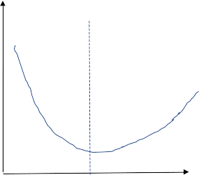
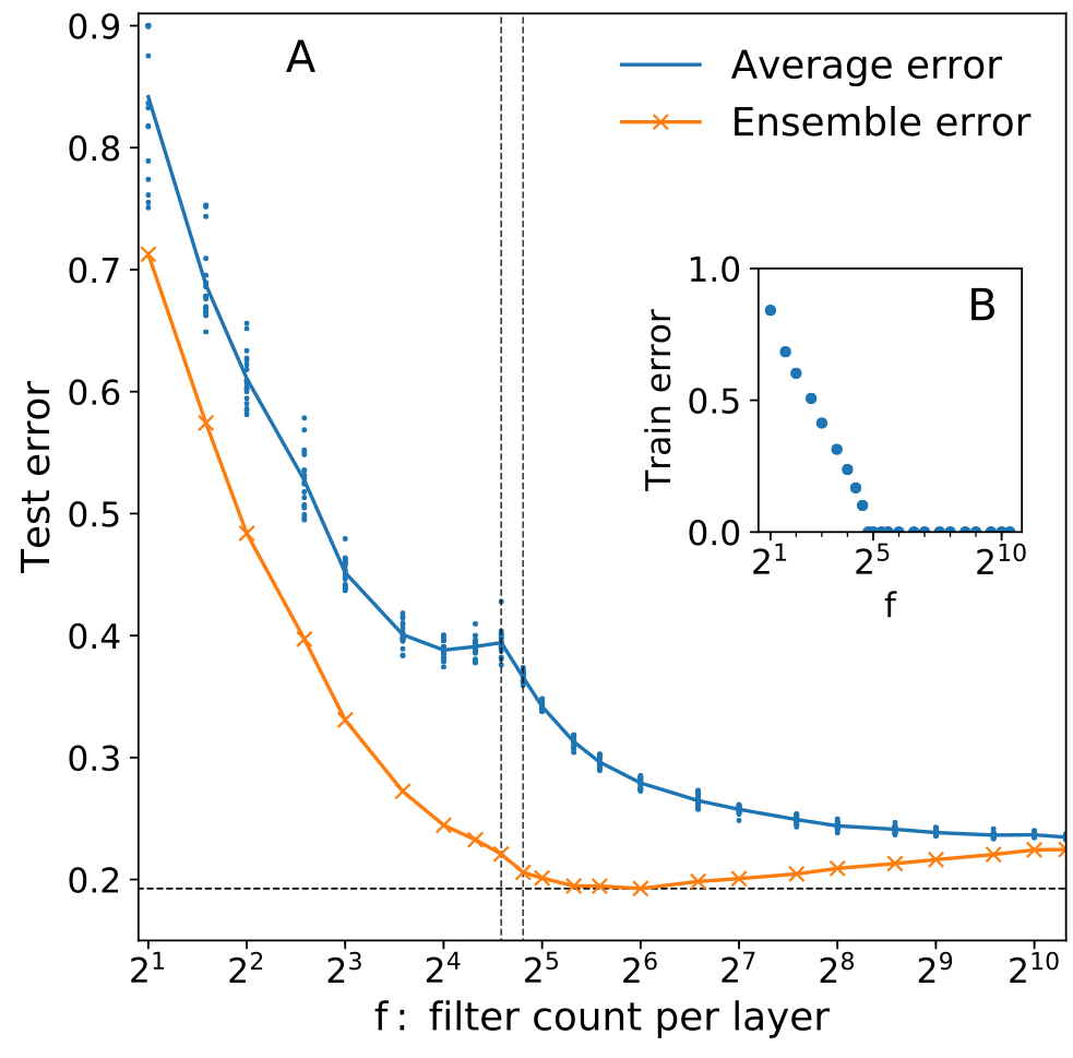
Overfitting?

Spigler et al. '18 - arXiv:1810.09665

Test error decreases monotonically with $N$!
Cusp at the jamming transition

Advani and Saxe '17;

Spigler et al. '18 - arXiv:1810.09665;

Geiger et al. '19 - arXiv:1901.01608

"Double descent"

test error

$N$

$N/N^*$

(after the peak)

$P$

$N$

dataset size

network size

We know why: Fluctuations!

Ensemble average

Random initialization $\to$ output function $f_{\color{red}N}$ is stochastic
Fluctuations: quantified by average and variance

ensemble average over $n$ instances:

\bar f^n_N(\mathbf{x}) \equiv \frac1n \sum_{\alpha=1}^n f_N(\mathbf{x}; \mathbf{W}_\alpha)

$\phantom{x}$

$f_N(\mathbf{W}_1)$

$f_N(\mathbf{W}_2)$

$f_N(\mathbf{W}_3)$

$-1$

$+1$

\overbrace{\phantom{wwwwwwwwwwwwwwwwi}}

$\bar f_N$

$-1!$

$\frac{{\color{red}-1-1}{\color{blue}+1}}{3}\cdots$

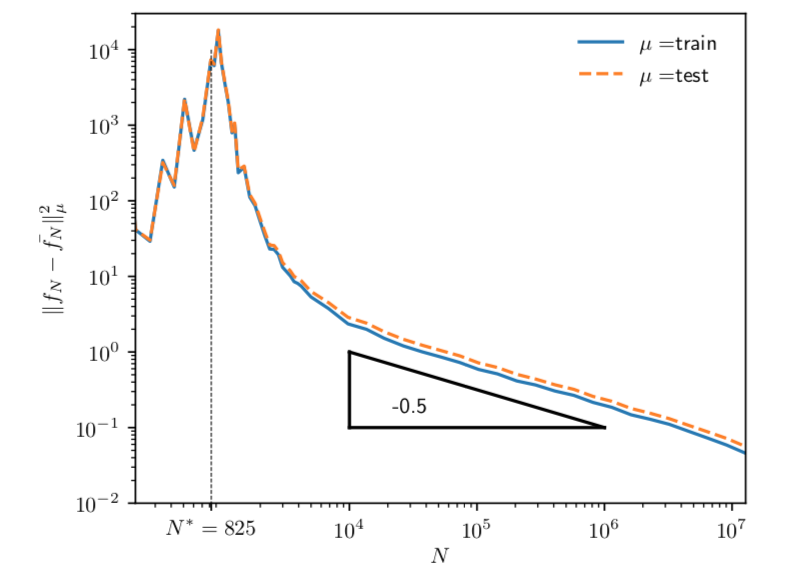
|\!|f_N - \bar f^n_N|\!|^2 \sim N^{-\frac12}

Explained in a few slides

Define some norm over the output functions:

ensemble variance (fixed $n$):

$\phantom{x}$

Fluctuations increase error

$ \{f(\mathbf{x};\mathbf{W}_\alpha)\} \to \left\langle\epsilon_N\right\rangle$

Remark:

Geiger et al. '19 - arXiv:1901.01608

Test error increases with fluctuations
Ensemble test error is nearly flat after $N^*$!

$\bar f^n_N(\mathbf{x}) \to \bar\epsilon_N$

test error of ensemble average

average test error

$\neq$

normal average

ensemble average

test error $\epsilon$

(CIFAR-10 $\to$ regrouped in 2 classes)

(MNIST parity)

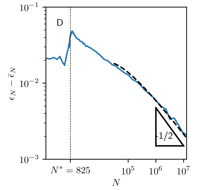
Scaling argument!

Geiger et al. '19 - arXiv:1901.01608

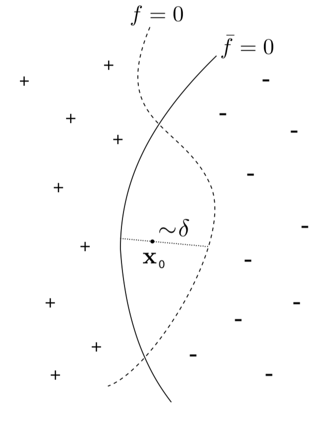
decision boundaries:

Smoothness of test error as function of decision boundary + symmetry:

\left\langle\epsilon_N\right\rangle - \bar\epsilon_N \sim |\!|f_N - \bar f_N|\!|^2 \sim N^{-\frac12}

normal average

ensemble average

Infinitely-wide networks: Initialization

Neal '96; Williams '98; Lee et al '18; Schoenholz et al. '16

Weights: each initialized as $W_\mu\sim {\color{red}h}^{-\frac12}\mathcal{N}(0,1)$
Neurons sum $\color{red}h$ signals of order ${\color{red}h}^{-\frac12}$ $\longrightarrow$ Central Limit Theorem
Output function becomes a Gaussian Random Field

width $\color{red}h$

$f(\mathbf{x};\mathbf{W})$

input dim $\color{red}d$

$W^{(1)}\sim d^{-\frac12}\mathcal{N}(0,1)$

as $h\to\infty$

$W_\mu$

Infinitely-wide networks: Learning

Jacot et al. '18

For small width $h$: $\nabla_{\mathbf{W}}f$ evolves during training
For large width $h$: $\nabla_{\mathbf{W}}f$ is constant during training

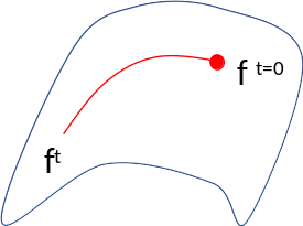
For an input $\mathbf{x}$ the function $f(\mathbf{x};\mathbf{W})$ lives on a curved manifold

The manifold becomes linear!

Lazy learning:

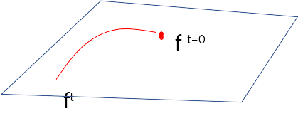
weights don't change much:
enough to change the output $f$ by $\sim \mathcal{O}(1)$! $\partial_{\mathbf{W}}$

|\!|\mathbf{W}^t - \mathbf{W}^{t=0}|\!|^2 \sim \frac1h

Neural Tangent Kernel

Gradient descent implies:

\displaystyle \frac{\mathrm{d}}{\mathrm{d}t} f(\mathbf{x}{\color{gray};\mathbf{W}^t}) = \sum_{i=1}^P \ \Theta^t(\mathbf{x},\mathbf{x}_i) \ \ {\color{gray} y_i \ell^\prime(y_i f(\mathbf{x}_i;\mathbf{W}^t))}

\Theta^t(\mathbf{x},\mathbf{x}^\prime) = \nabla_{\mathbf{W}} f(\mathbf{x}{\color{gray};\mathbf{W}^t}) \cdot \nabla_{\mathbf{W}} f(\mathbf{x}^\prime{\color{gray};\mathbf{W}^t})

The formula for the kernel $\Theta^t$ is useless, unless...

Theorem. (informal)

\lim_{\mathrm{width}\ h\to\infty} \Theta^t(\mathbf{x},\mathbf{x}^\prime) \equiv \Theta_\infty(\mathbf{x},\mathbf{x}^\prime)

Deep learning $=$ learning with a kernel as $h\to\infty$

Jacot et al. '18

$\phantom{x}$

\overbrace{\phantom{wwwwwwwwwwwwwwwwwwi}}

convolution with a kernel

$\phantom{wwwwwwww}$

Finite $N$ asymptotics?

Geiger et al. '19 - arXiv:1901.01608;

Hanin and Nica '19;

Dyer and Gur-Ari '19

Evolution in time is small:
Fluctuations are much larger:

Then:

|\!|f_N-\bar f_N|\!|^2 \sim \left(\Delta\Theta^{t=0}\right)^2 \sim N^{-\frac12}

The output function fluctuates similarly to the kernel

$\Delta\Theta^{t=0} \sim 1/\sqrt{h} \sim N^{-\frac14}$

at $t=0$

$|\!|\Theta^t - \Theta^{t=0}|\!|_F \sim 1/h \sim N^{-\frac12}$

\displaystyle f(\mathbf{x}{\color{gray};\mathbf{W}^t}) = \int \mathrm{d}t \sum_{i=1}^P \ \Theta^t(\mathbf{x},\mathbf{x}_i) \ \ {\color{gray} y_i \ell^\prime(y_i f(\mathbf{x}_i;\mathbf{W}^t))}

Conclusion

1. Can networks fit all the $\color{red}P$ training data?

Yes, deep networks fit all data if $N>N^*\ \longrightarrow$ jamming transition
Initialization induces fluctuations in output that increase test error
No overfitting: error keeps decreasing past $N^*$ because fluctuations diminish

check Geiger et al. '19 - arXiv:1906.08034 for more!

check Spigler et al. '19 - arXiv:1905.10843 !

2. Can networks overfit? Can $\color{red}N$ be too large?

3. How does the test error scale with $\color{red}P$?

$\to$ Long term goal: how to choose $\color{red}N$?

(tentative) Right after jamming, and do ensemble averaging!

Loss Landscape and Performance in Deep Learning

By Stefano Spigler

Loss Landscape and Performance in Deep Learning

Talk given in ICTS, Bangalore, January 2020

Stefano Spigler

spigler.net/stefano

Loss Landscape and

Performance in Deep Learning

(Supervised) Deep Learning

Set-up: Architecture

Set-up: Dataset

Outline

Learning

Learning dynamics = descent in loss landscape

Analogy with granular matter: Jamming

Theoretical results: Phase diagram

Empirical tests: MNIST (parity)

Landscape curvature

Flat directions

Outline

Generalization

Overfitting?

Ensemble average

Fluctuations increase error

Scaling argument!

Infinitely-wide networks: Initialization

Infinitely-wide networks: Learning

Neural Tangent Kernel

Finite \(N\) asymptotics?

Conclusion

Loss Landscape and Performance in Deep Learning

More from Stefano Spigler