Data Science 101
Linear and logistic regression
Outline
- Linear Regression
- In practice
- Logistic Regression
- Model
- Cost and optimisation
- Multi-classification
Linear regression
Last week
Our first supervised model with the hypothesis:
\( h(x) = \theta_0 + \theta_1 x \)
We have a function ("cost function") to evaluate this model error:
And an algorithm to minimize this function in order to get the best parameters \( \theta_0, \theta_1 \):
Repeat until convergence {
}
J(\theta_0, \theta_1) = \frac{1}{n}
\displaystyle\sum_{i=1}^{n} (h(x_i) - y_i)^2
\theta_j := \theta_j - \alpha \frac{\partial}{\partial \theta_j} J(\theta_0, \theta_1)
Before
| Size | Price |
|---|---|
| 1060 | 244 |
| 920 | 231 |
| 250 | 76 |
| ... | ... |
h(x) = \theta_0 + \theta_1 x
Reality
| Size | # of bedrooms | # of floors | Age of home | ... | Price |
|---|---|---|---|---|---|
| 1060 | 5 | 2 | 40 | ... | 244 |
| 920 | 3 | 1 | 32 | ... | 231 |
| 750 | 4 | 2 | 15 | ... | 197 |
| ... | ... | ... | ... | ... | ... |
\( x \) (features)
\( y \) (target)
Reality
| Size | # of bedrooms | # of floors | Age of home | Price |
|---|---|---|---|---|
| 1060 | 5 | 2 | 40 | 244 |
| 920 | 3 | 1 | 32 | 231 |
| 750 | 4 | 2 | 15 | 197 |
| ... | ... | ... | ... | ... |
Notation:
\( n \) = Number of training examples
\( m \) = Number of features
\( x \) = Matrice "input" variable / features
\( x_i \) = \( i^{th} \) column of x
\( y \) = "output" variable / "target" variable
Training set: \( n \times m \) matrix
Hypothesis
h(x) = \theta_0 + \theta_1 x_1 + \theta_2 x_2 + ... + \theta_m x_m
For convenience of notation, define \( x_0 = 1 \):
h(x) = \theta^T x
J(\theta) = \frac{1}{n}
\displaystyle\sum_{i=1}^{n} (h(x_i) - y_i)^2
Cost function & Gradient descent
\theta_j := \theta_j - \alpha \frac{\partial}{\partial \theta_j} J(\theta)
Repeat until convergence {
}
In pratice
First steps in feature engineering
Feature Scaling: Idea
Make sure features are on a similar scale
| Size | # bedrooms |
|---|---|
| 1060 | 2 |
| 920 | 4 |
| 250 | 1 |
Example:
\( x_1 \): size (0-1000)
\( x_2 \): # of bedrooms (1- 4)
Variation of \( \theta_2 \) will impact a lot the value of \( J(\theta) \) compared to \( \theta_1 \)
=> We want to put everything at better scale (ie. between some interval)
Rescaling
Simpliest method, rescale to the range [0, 1]:
x' = \frac{x - min(x)}{max(x) - min(x)}
| Size |
|---|
| 1060 |
| 920 |
| 250 |
| Size' |
|---|
| 1 |
| 0.83 |
| 0 |
Mean normalization
x' = \frac{x - \bar{x}}{max(x) - min(x)}
| Size |
|---|
| 1060 |
| 920 |
| 250 |
| Size' |
|---|
| 0.39 |
| 0.22 |
| -0.62 |
Standardization
Remove the mean and unit variance
x' = \frac{x - \bar{x}}{\sigma}
std = \sqrt{var} = \sigma = \sqrt{\frac{\displaystyle\sum_{i=1}^{n}(x_i - \bar{x})^2}{n - 1}}
Standardization
Remove the mean and unit variance
x' = \frac{x - \bar{x}}{\sigma}
| Size |
|---|
| 1060 |
| 920 |
| 250 |
| Size' |
|---|
| 0.89 |
| 0.49 |
| -1.39 |
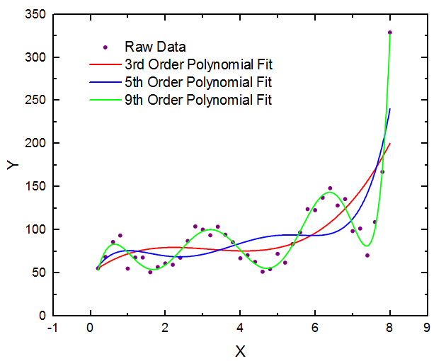
Polynomial features
Duplicate some feature with their degree
Example:
\( \theta_0 + \theta_1 x_1 \)
Second degree: \( \theta_0 + \theta_1 x_1 + \theta_2 x_1^2 \)
Third degree: \( \theta_0 + \theta_1 x_1 + \theta_2 x_1^2 + \theta_3 x_1^3 \)
...
Polynomial features
Logistic regression
Model
Binary classification
Email: Spam or not spam?
Tumor: Malignant or benign?
Sport: Will a team win a next game?
Output is:
\( y \in \{0,1\} \)
0 is the "negative" class
1 is the "positive" class
Intuition
Given some data, we want to predict the probability of an output.
For example, given the score of a team, what is the probability it will win.
\( 0 < p( win\) | \(score ) < 1 \)
If p(win|score) > 0.5 then predict "Win" ("1") else "Loose" ("0")
We want our model to reflect this and outputs in [0,1]
Our example:
Will a team win?

Linear Regression

Sigmoid
g(z) = \frac{1}{1 + e^{-z}}
Sigmoid
g(z) = \frac{1}{1 + e^{-z}}
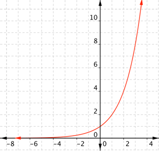
Exponential:
Sigmoid

g(z) = \frac{1}{1 + e^{-z}}
Logistic Regression
h(x) = g(\theta^T x) = \frac{1}{1 + e^{-\theta^T x}}
With g = the sigmoid function
h(x) = p(y=1|x;\theta)
"Probability that y = 1, given x, parameterized by \( \theta \)"
Logistic regression
Cost function & optimisation
Loss function in general
J(\theta) = \frac{1}{n}
\displaystyle\sum_{i=1}^{n} cost(h(x_i), y_i)
cost(h(x_i), y_i) = (h(x_i) - y_i)^2
For the linear regression, we saw the cost function named "Mean squared error":
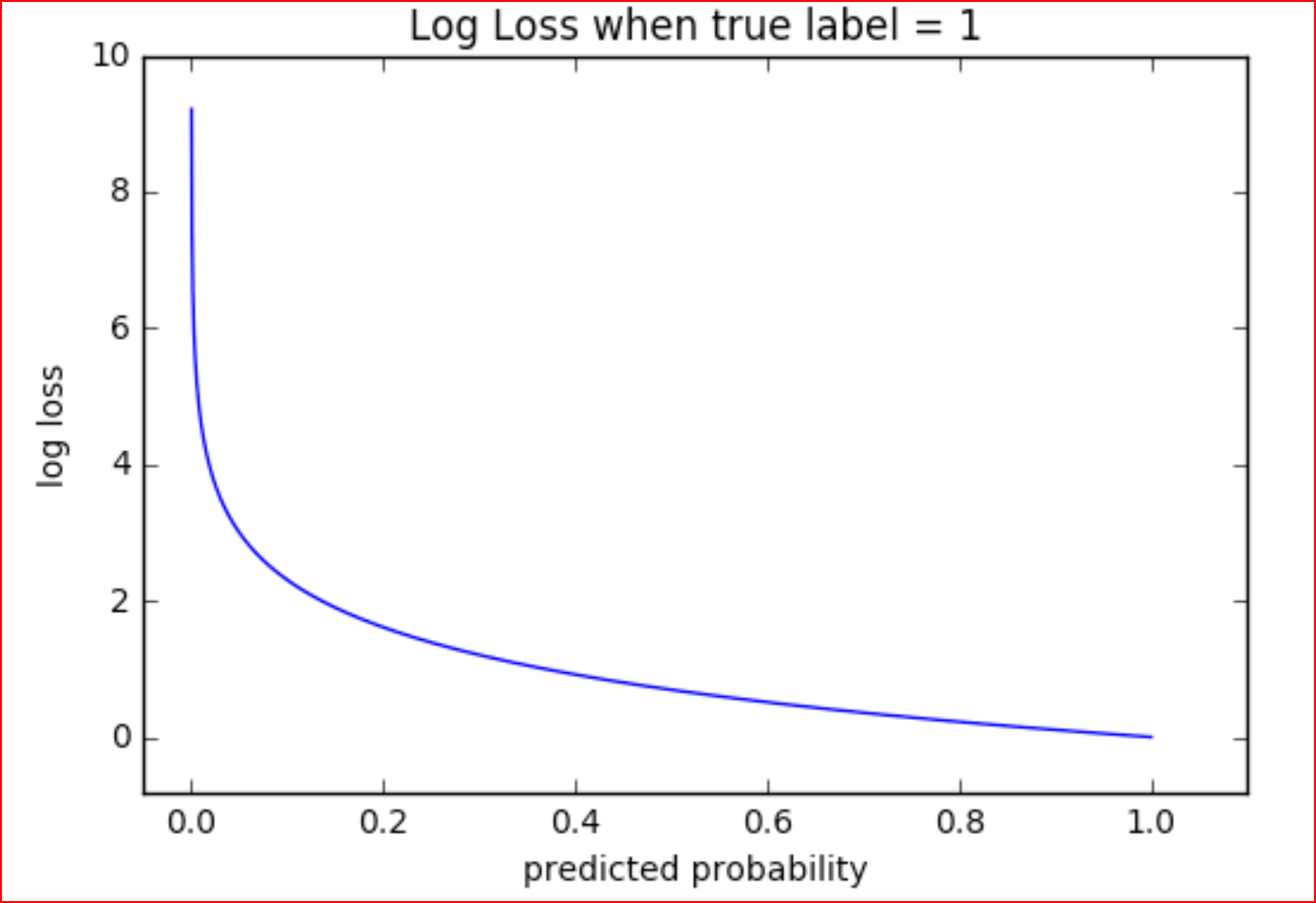
Logarithmic Loss
The loss to a certain predicted probability \( p \) in regard to the truth \( y \)
LogLoss(y, p) = y \space log \space p
Logarithmic Loss
The loss to a certain predicted probability \( p \) in regard to the truth \( y \)
LogLoss(y, p) = y \space log \space p
LogLoss(1, 0.9) = 0.10536
Examples:
LogLoss(1, 0.5) = 0.69315
LogLoss(1, 0.1) = 2.3026
Logarithmic Loss
Logarithmic Loss
J(\theta) = - \frac{1}{n}
\displaystyle\sum_{i=1}^{n} y_i \space log \space h(x_i) + (1 - y_i) \space log(1 - h(x_i))
0 if the current sample \( i \) has a negative output
\( y = 0 \)
0 if the current sample \( i \) has a positive output
\( y = 1 \)
Gradient Descent
Nothing really change!
Repeat until convergence {
}
\theta_j := \theta_j - \alpha \frac{\partial}{\partial \theta_j} J(\theta)
Just compute the partial derivative of our new cost function
Multi-classification
One vs All

One vs All
For \(K \) classes, \( j = 1 \space ... \space K \)
Train multiple classifier \( h_j(x) \) for each class \( j \)
On a new input \( x \), to make a new prediction, pick the class \( j \) that maximes:
$$ \max_{j} h(x) $$
Code
Linear Regression
from sklearn import linear_model

ols = linear_model.LinearRegression()

ols.fit(X, y)       # Train your model
ols.coef_           # Theta
ols.predict(X_new)  # Predict on a new value
from sklearn import linear_model
clf = linear_model.LogisticRegression()
clf.fit(X, y) # Train your model
clf.coef_ # Theta
clf.predict(X_new) # Predict on a new valueLogistic Regression
Where are we?
Now
You know how to solve a regression and classification model with a linear model.
You also know how to rescale features.
What you miss to work on your first problem
Next session, we will learn how to train and evaluate a model properly in practice.
And how to tackle some common problems (overfitting, CV,...)
What's next
After that, for supervised learning, it all will be new models, optimisation methods, tricks to tackle specific problems: imbalanced learning, dealing with text data, image data,...
Internal competition(s) ?
Kaggle Inclass
Regression: Predict NYC house price
Classification: Predict if a patient has a disease or not
Multi-Classification: Predict if a water pump in Africa is functional, need some repairs or don't work at all
Data science 101.2
By Yann Carbonne


