DeepRetina
Yigit DEMIRAG
Reyhan ERGUN
Gokhan GOK
Neural Network Performances on
MNIST Handwritten Digits Database
BILKENT - 2015
Outline
- MNIST Database
- kNN, SVM
- Two Layer Feed Forward Network
- Convolutional Neural Network
- Convolutional Deep Neural Networks
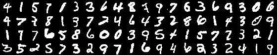
MNIST Database
- 60k training, 10k test images
- 28x28 pixel size
- Black/White, size-normalized and centered.
- Currently one of the leading database for testing neural networks (CIFAR-10, SVHN etc.)
k-Nearest Neighbourhood
- No training required.
- Algorithm:
Input: D, the set of K-training objects, and test object
Process:
Compute , the distance between z and every object,
Select , the set of k closest training objects to z.
Output:
(x,y) \in D
d(x',x)
z= (x',y')
D_z \subseteq D
y' = \arg\max_{v} \Sigma_{(x_i,y_i) \in D} I(v= y_i)
k-Nearest Neighbourhood - Results
Accuracy : 96.13%
k-Nearest Neighbourhood - Results
Pros:
- High accuracy
- Insensitive to outliers
- No assumption to data
Cons:
- Computationally expensive
- Requires a lot memory
- No hierarchical structure is captured.
SVM - Calculations
- Instead of dealing P, we deal with D (used MATLAB quadprog(), input matrix, and vectors calculated as shown in our lecture)
- Determined the optimum Lagrange multipliers
i.e. from the result of quadprog().
- Compute the optimum weight vector as
- Compute the optimum bias as
- Average found for each SV, (since we obtained a different for each SV)
\alpha_{o,i}
\mathbf{w_o} = \sum\limits_{i=1}^{N_s} \alpha_{o,i} d_i \mathbf{x}_i
b_o = 1 - \mathbf{w}_o^T \mathbf{x}^{(s)}
\text{ for } d^{(s)} = 1
= 1 - \sum\limits_{i=1}^{N_s} \alpha_{o,i} d_i \mathbf{x}_i^T \mathbf{x}^{(s)}
b_o
b_o
SVM - Setup
2. Used as one vs rest classifier to deal with less number of SVMs.
3. 4000 training data with equally likely distribution.
4. Used highest probability result when more than one binary SVM
estimated a label.
5. Used highest probability "non reported" result when none of the
binary SVM estimated a label.
SVM - Results
| N | T | SV | L | Acc | |
|---|---|---|---|---|---|
| Label 0 vs Rest | 4000 | 500 | 2760 | Inf | |
| Label 1 vs Rest | 4000 | 500 | 431 | Inf | |
| Label 2 vs Rest | 4000 | 500 | 2996 | Inf | |
| Label 3 vs Rest | 4000 | 500 | 4000 | Inf | |
| Label 4 vs Rest | 4000 | 500 | 3638 | Inf | |
| Label 5 vs Rest | 4000 | 500 | 3998 | Inf | |
| Label 6 vs Rest | 4000 | 500 | 3445 | Inf | |
| Label 7 vs Rest | 4000 | 500 | 3330 | Inf | |
| Label 8 vs Rest | 4000 | 500 | 4000 | Inf | |
| Label 9 vs Rest | 4000 | 500 | 4000 | Inf | |
| Overall | 4000 | 500 | - | Inf | 46.6 |
SVM - Results
| N | T | SV | L | Acc | |
|---|---|---|---|---|---|
| Train data from 1st 4000 | 4000 | 500 | - | Inf | 22.28 |
| Train data from 2nd 4000 | 4000 | 500 | - | Inf | 22.24 |
| Train data from 3rd 4000 | 4000 | 500 | - | Inf | 46 |
| Train data from 4th 4000 | 4000 | 500 | - | Inf | 34.2 |
| Train data from 5th 4000 | 4000 | 500 | - | Inf | 41.8 |
| Train data from 6th 4000 | 4000 | 500 | - | Inf | 44.5 |
SVM - Results
Pros
1. Achieves a maximum separation of the data, i.e., "optimal separating hyper-plane"
2. It can deal with very high dimensional data.
3. Computational complexity less when compared with kNN*
4. Use of "kernel trick"**
Cons
1. *But as in our case, when number of SVs are high computational complexity increases. (when training data gets larger, number of SVs get larger)
2. **Need to select a good kernel function (should add new features so that we have a linearly separable data set from)
Two Layer Feedforward Neural Network - Setup
F.c. Layer - F.c. Layer
- Written in Python.
- Optimized via SGD.
- Batch size is 100.
- # of epoch is 200.
- Trained/Tested on EC2 with 32 CPUs.
Two Layer Feedforward Neural Network - Setup
| Hyper Parameters | Value |
|---|---|
| Regularization | 1 |
| Learning Rate | 1e-5 |
| # of Hidden Units | 300 |
| Momentum | 0.98 |
| Activation Func. | ReLU |
| Cost | Cross-entropy + reg. |
F.c. Layer - F.c. Layer
Two Layer Feedforward Neural Network - Setup
Result
89.83%
Convolutional Neural Network
Conv - Pool - F.c. Layer
- Written in MATLAB.
- Optimized via SGD.
- Batch size is 256.
- # of epoch is 10.
Convolutional Neural Network
Conv - Pool - F.c. Layer
| Hyper Parameters | Value |
|---|---|
| Filter Width | 9 |
| Pooling Size | 2x2 |
| Learning Rate | 0.1 |
| # of Features | 20 |
| Momentum | 0.95 |
| Activation Func. | Softmax |
| Cost | Cross ent. + Reg. |
Convolutional Neural Network - Model Comparison
| Kernel Width | 7 | 9 | 11 |
|---|---|---|---|
| Accuracy | 98.2% | 98.08% | 98.2% |
| # of Kernels | 14 | 16 | 18 | 20 | 22 | 24 | 26 | 28 |
|---|---|---|---|---|---|---|---|---|
| Accuracy | 98.4% | 98.2% | 98.4% | 98.1% | 98.3% | 98.3% | 98% | 98.3% |
| Momentum | 0.2 | 0.4 | 0.6 | 0.8 | 0.9 | 0.95 |
|---|---|---|---|---|---|---|
| Accuracy | 96.5% | 96.6% | 97.4% | 97.9% | 98% | 98.5% |
Best Result: 98.08%
Deep Convolutional Neural Network
Conv. - Pool - Conv. - Pool - F.c. Layer - F.c. Layer
- Written in Torch7.
- Optimized via SGD.
- Batch size is 100.
- # of epoch is 100.
- Learning rate 0.05
- Trained/Tested on nVIDIA GTX on EC2.
Deep Convolutional Neural Network - Activation Functions
| Activation Func. | Accuracy |
|---|---|
| Tanh | 99.14% |
| ReLU | 99.18% |
| Sigmoid | 98.77% (Takes too long!) |

Deep Convolutional Neural Network - Momentum
| Momentum | Accuracy |
|---|---|
| 0.95 | 99.12% |
| 0.90 | 99.08% |
| 0.98 | 98.84% |

Deep Convolutional Neural Network - Dropout
| Dropout | Accuracy |
|---|---|
| 0.2 | 98.86% |
| 0.4 | 98.92% |
| 0.6 | 97.74% |
Deep Convolutional Neural Network - More Deeper Models
| Activation Func. | Dropout | Momentum | Accuracy |
|---|---|---|---|
| ReLU | - | - | 99.15% |
| Tanh | - | - | 98.97% |
| ReLU | 0.4 | - | 98.84% |
| ReLU | 0.2 | - | 98.86% |
| ReLU | - | .95 | 99.21% |
| ReLU | - | .98 | 99.09% |
Conv. - Pool - Conv. - Pool - F.c. Layer - F.c. Layer - F.c. Layer
Deep Convolutional Neural Network - Batch Normalization
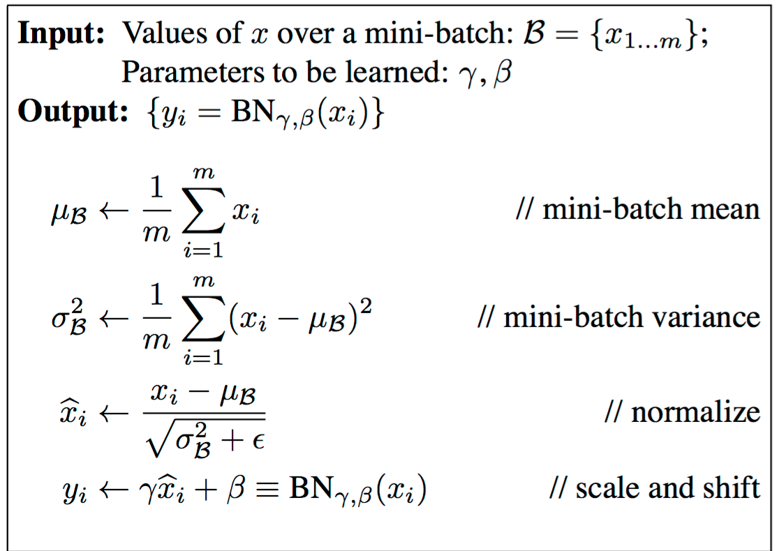
- In SGD , the distribution of inputs to a hidden layer will change because the hidden layer before it is constantly changing as well. This is known as covariate shift.
- It is known that whitened data makes learning faster.
- Therefore apply whitening to every layer.
| (arXiv:1502.03167 [cs.LG]) |
Deep Convolutional Neural Network - Batch Normalization

Deep Convolutional Neural Network - Batch Normalization
| Batch Normalization | Accuracy |
|---|---|
| 2 F.c. Layer | 98.86% |
| 3 F.c. Layer | 98.85% |
| 4 F.c. Layer (+.95 momentum) | 98.79% |

Deep Convolutional Neural Network - More Deeper Models
| Activation Func. | Dropout | Momentum | Accuracy |
|---|---|---|---|
| ReLU | - | .95 | 99.31% |
Conv. - Pool - Conv. - Pool - F.c. Layer - F.c. Layer - F.c. Layer - F.c. Layer
Deep Convolutional Neural Network - Practical Issues
- For the search of the best model, one should run several different models at the same time.
- This requires high computing resource.
- GPUs are ~x10 faster than CPUs.
- Google's Tensorflow does not work on Amazon GPUs.
- Sigmoid is not useful as it is x10-15 times slower than ReLU, tanh.
- Dropout did not give much benefit.
Final Result
99.31\%
Conv - Pool - Conv - Pool - F.c Layer - F.c. Layer - F.c. Layer - F.c. Layer
ReLU
.95 Momentum
No Dropout
Thanks for Listening!
DeepRetina
DeepRetina Final Presentation
By Yigit Demirag