Interaction driven topological superconductivity
Zhi Han, Joseph Maciejko

Roadmap
- Majorana particles
- The Kitaev chain
- The Interaction Hamiltonian
- Results
In quantum mechanics and quantum field theory, the creation and destruction operators for fermions (in momentum space) are:
c^{\dagger} c+c c^{\dagger}=1 \quad c^2 = \left(c^\dagger \right)^2 = 0
c^\dagger|0\rangle = |1\rangle \quad c|1\rangle = |0\rangle
Creation and Destruction
c|0\rangle= 0 \quad c^{\dagger}|1\rangle= 0
This can be neatly summed up by the following rules:
c^{\dagger} c+c c^{\dagger}=1 \quad c^2 = \left(c^\dagger \right)^2 = 0
Creation and Destruction 2
But for multiple particles, we have: (using the anticommutator:)
\begin{aligned}\left\{c_{i}, c_{j}^{\dagger}\right\} & \equiv c_{i} c_{j}^{\dagger}+c_{j}^{\dagger} c_{i}=\delta_{i j} \\\left\{c_{i}^{\dagger}, c_{j}^{\dagger}\right\} &=\left\{c_{i}, c_{j}\right\}=0 \end{aligned}
For a single fermion, we have:
When you have a pair of creation and destruction operators, you can write down the following unitary transformation:
c^{\dagger}=\frac{1}{2}\left(\gamma_{1}+i \gamma_{2}\right), \quad c=\frac{1}{2}\left(\gamma_{1}-i \gamma_{2}\right)
A unitary transformation
The pair \(\gamma_1\) and \(\gamma_2\) are called Majorana operators. Notice that \(\gamma\) = \(\gamma^\dagger\). We can check that Majoranas satisfy the following conditions:
\gamma_{1} \gamma_{2}+\gamma_{2} \gamma_{1}=0, \gamma_{1}^{2}=1, \gamma_{2}^{2}=1
\gamma_{1} \gamma_{2}+\gamma_{2} \gamma_{1}=0, \gamma_{1}^{2}=1, \gamma_{2}^{2}=1
Multiple Majoranas
For a single particle:
For multiple particles, we can also check that:
\left\{\gamma_{i}, \gamma_{j}\right\} \equiv \gamma_{i} \gamma_{j}^{\dagger}+\gamma_{j}^{\dagger} \gamma_{i}=2\delta_{i j}
\begin{aligned}\left\{c_{i}, c_{j}^{\dagger}\right\} & \equiv c_{i} c_{j}^{\dagger}+c_{j}^{\dagger} c_{i}=\delta_{i j} \\\left\{c_{i}^{\dagger}, c_{j}^{\dagger}\right\} &=\left\{c_{i}, c_{j}\right\}=0 \end{aligned}
Compare this to the many-body fermion algebra:
Does this mean we just found a particle that is it's own antiparticle? This is the theoretical prediction made by Ettore Majorana in 1937.
Majorana particles?

How to generate Majoranas
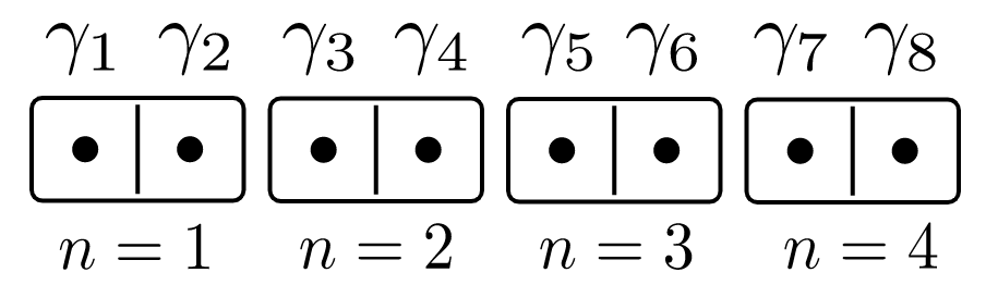
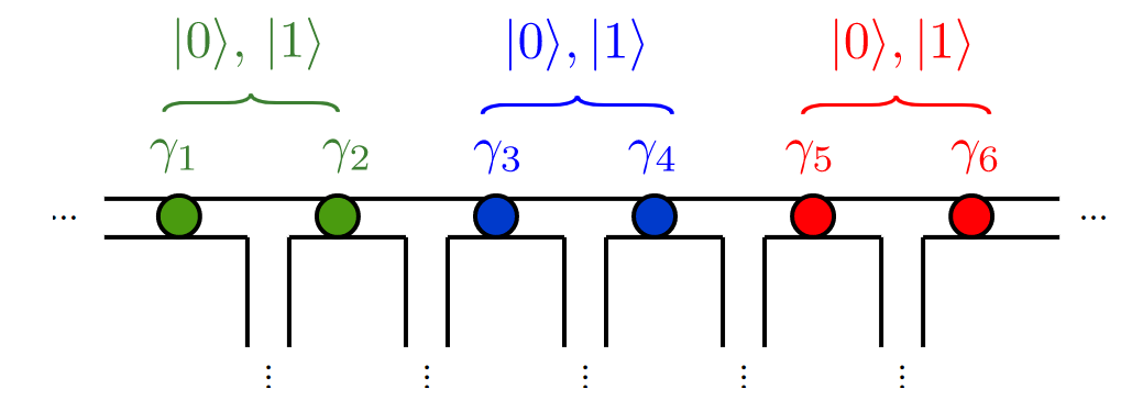
One proposed model containing Majoranas is the Kitaev chain. The Kitaev chain is just \(n\) electrons in a row:
The Trivial Phase
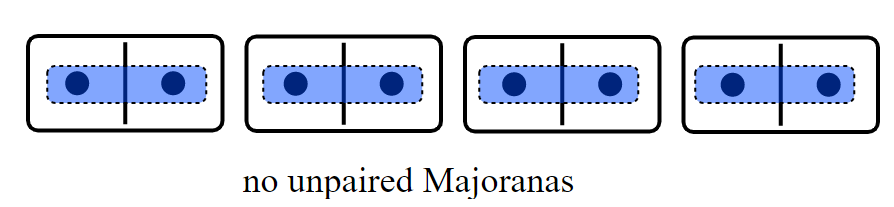
We can pair them like this:
H=(i / 2) \mu \sum_{n=1}^{N} \gamma_{2 n-1} \gamma_{2 n}
Each majorana having energy \(\mu/2\):
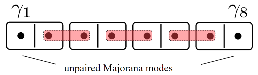
The Topological Phase
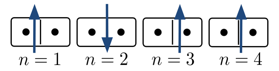
Or like this, each Majorana having an energy \(t\):
Text
H=i t \sum_{n=1}^{N-1} \gamma_{2 n} \gamma_{2 n+1}
The Kitaev Chain
H=-\mu \sum_{n} c_{n}^{\dagger} c_{n}-t \sum_{n}\left(c_{n+1}^{\dagger} c_{n}+\mathrm{h.c.}\right)+\Delta \sum_{n}\left(c_{n} c_{n+1}+\mathrm{h.c.}\right)
We can put it into one Hamiltonian, and converting back from Majoranas to electrons we obtain the model of the Kitaev chain:
-
\(\mu\) is the chemical potential
-
\(t\) is the kinetic energy
-
\(\Delta\) is the superconducting band gap
Quantum Phase Transition!
Why do we care?
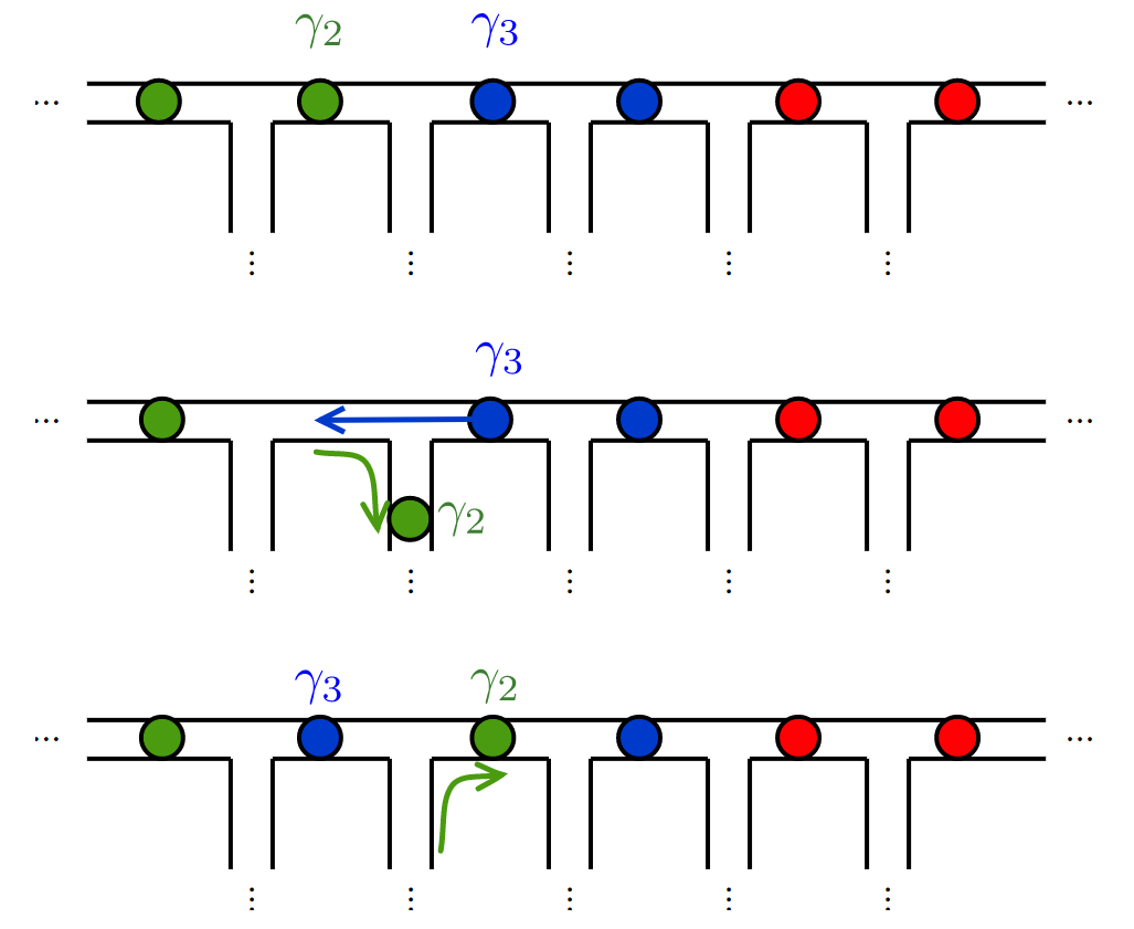
The Majoranas are a topological property of the system. Therefore if we slice off the Kitaev Chain, a new Majorana will appear.
These are the ideas behind topological quantum computing:
1.Topology protects the system against decoherence
2. We can store information inside phase state of the Kitaev chain
3. Computing is done using cool Majorana tricks
Aside: Topological quantum computing
Computations are "closed loops"
Non abelian statistics
Majoranas are "anyons", neither bosons nor fermions
Topology as emergent behaviour?
Okay. I'm on board. How do we get a Kitaev chain.
The question we would like to answer is can topology and exotic particles arise out of just electron interactions?
The Kitaev chain does not take spin interactions into account. Adding them in, we get our interaction-driven Hamiltonian!
Ising Model
In the Ising model, there is a quantum phase transition from to \({\sigma^z}_{i, i+1} = 0\) (Paramagnetism). \({\sigma^z}_{i, i+1} = 1\) (Ferromagnetism). Hence, we should expect a quantum phase transition for the interaction-driven Hamiltonian as well.
The Ising model describes "spins in a chain". The Hamiltonian is given as follows:
H=-J \sum_{i} \sigma_{i, i+1}^{z} \sigma_{i+1, i+2}^{z}-h \sum_{i} \sigma_{i, i+1}^{x}
\({\sigma^z}_{i, i+1} = 1\) (Ferromagnetism)
\({\sigma^z}_{i, i+1} = 0\) (Paramagnetism)
The interaction driven Hamiltonian
Our Hamiltonian consists of N electrons on a 1D lattice, with spins \(\sigma_{i, i+1}\) living on the nearest-neighbour bonds of this lattice. The Hamiltonian is
•\(J\) - spin interaction
•\(h\) - randomization noise
•\(\Delta\) - superconducting band gap
•\(\mu\) - chemical potential
•\(t\) - kinetic energy/hopping
H=-t \sum_{i}\left(c_{i}^{\dagger} c_{i+1}+\mathrm{h.c.}\right)-\mu \sum_{i} c_{i}^{\dagger} c_{i} \quad+\Delta \sum_{i}\left(c_{i} \sigma_{i, i+1}^{z} c_{i+1}+\mathrm{h.c.}\right) -J \sum_{i} \sigma_{i, i+1}^{z} \sigma_{i+1, i+2}^{z}-h \sum_{i} \sigma_{i, i+1}^{x}
Limiting cases: topological
H=-t \sum_{i}\left(c_{i}^{\dagger} c_{i+1}+\mathrm{h.c.}\right)-\mu \sum_{i} c_{i}^{\dagger} c_{i} \quad+\Delta \sum_{i}\left(c_{i} \sigma_{i, i+1}^{z} c_{i+1}+\mathrm{h.c.}\right) -J \sum_{i} \sigma_{i, i+1}^{z} \sigma_{i+1, i+2}^{z}-h \sum_{i} \sigma_{i, i+1}^{x}
Limiting cases: If \(\sigma^z_{i, i+1} = 1\) and \( h\) is small we get back the Kitaev Chain.
H_{Kitaev}=-\mu \sum_{n} c_{n}^{\dagger} c_{n}-t \sum_{n}\left(c_{n+1}^{\dagger} c_{n}+\mathrm{h.c.}\right)+\Delta \sum_{n}\left(c_{n} c_{n+1}+\mathrm{h.c.}\right)
Limiting cases: If \(\sigma^z_{i, i+1} = 1\) and \( h\) is small we get back the Kitaev Chain.
The topological phase cooresponds to \( \left\langle\sigma_{i, i+1}^{z}\right\rangle \neq 0\), and \(J/h \) large.
Recall the interaction Hamiltonian is:
Limiting cases: trivial
H=-t \sum_{i}\left(c_{i}^{\dagger} c_{i+1}+\mathrm{h.c.}\right)-\mu \sum_{i} c_{i}^{\dagger} c_{i} \quad+\Delta \sum_{i}\left(c_{i} \sigma_{i, i+1}^{z} c_{i+1}+\mathrm{h.c.}\right) -J \sum_{i} \sigma_{i, i+1}^{z} \sigma_{i+1, i+2}^{z}-h \sum_{i} \sigma_{i, i+1}^{x}
H_{metal}=-t \sum_{i}\left(c_{i}^{\dagger} c_{i+1}+\mathrm{h.c.}\right)-\mu \sum_{i} c_{i}^{\dagger} c_{i} + -J \sum_{i} \sigma_{i, i+1}^{z} \sigma_{i+1, i+2}^{z}-h \sum_{i} \sigma_{i, i+1}^{x}
The trivial phase cooresponds to \( \left\langle\sigma_{i, i+1}^{z}\right\rangle = 0\), and \(J/h \) large.
However, if \( \left\langle\sigma_{i, i+1}^{z}\right\rangle= 0\), the \( \Delta \) term disappears:
The four terms are nothing special, this is just a metal, or the trivial phase:
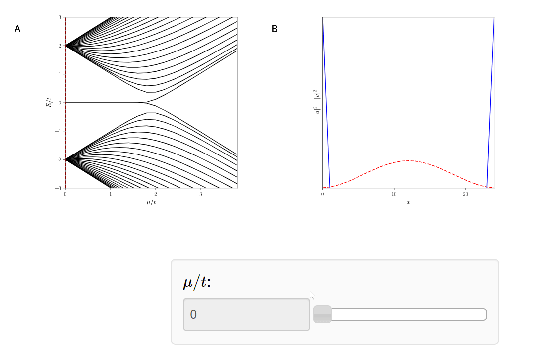
Method 1: Brute force exact diagonalization
Recall our goal is to compute the phase diagram for the interaction driven Hamiltonian.
- Numerical approach: "Plug and chug"
- Bad: Can only compute up to \(N=6\) particles, Hilbert space is size \(2^{2N} \)
- Smarter numerical approach: "Use symmetries to reduce computation, then plug and chug"
- We can rewrite this as a Bogoliubov-de Gennes Hamiltonian, which has particle hole symmetry. Then diagonalize.
- Bad: Can only do this in the case \(h=0 \), Hilbert space is size \( 2^N \)
import quspin
from scipy.linalg import eigsh

def make_Hamiltonian(N,J,h,t,mu,Delta):
    """Returns a Quantum Hamiltonian."""
    # Spin Hamiltonian
    J_sum = [[-J, i, (i+1)%N] for i in range(N)]
    h_sum = [[-h, i] for i in range(N)]

    # Fermion Hamiltonian
    t_sum_pm = [[-t, i,(i+1)%N] for i in range(N)]
    t_sum_mp = [[-t, (i+1)%N,i] for i in range(N)]
    mu_sum = [[-mu,i] for i in range(N)]
    Delta_sum_zmm = [[Delta, i,i,(i+1)%N] for i in range(N)]
    Delta_sum_zpp = [[Delta, i,(i+1)%N,i] for i in range(N)]

    static = [
        ["zz|",J_sum],
        ["x|",h_sum],
        ["|+-",t_sum_pm],
        ["|+-",t_sum_mp],
        ["z|--",Delta_sum_zmm],
        ["z|++",Delta_sum_zpp],
        ['|n',mu_sum]
    ]
    dynamic = []

    spin_basis = quspin.basis.spin_basis_1d(N)
    fermion_basis = quspin.basis.spinless_fermion_basis_1d(N)
    tensor_basis = quspin.basis.tensor_basis(spin_basis,fermion_basis) #spin | fermion

    no_checks = dict(check_pcon=False,check_symm=False,check_herm=False)

    H = quspin.operators.hamiltonian(static,dynamic,basis=tensor_basis,**no_checks)
    return H #returns as a Quspin Hamiltonian

H = make_Hamiltonian()
E, V = eigsh(H)
Method 2: The variational method
Use the variational method from Griffths Chapter 7.
The variational method:
1. Guess a wavefunction, will probably overestimate the ground state energy
2. Minimize the energy w.r.t that wavefunction
3. Take thermodynamic limit
Mean field approximation: \( \sigma_{i, i+1}^z=\left\langle\sigma_{i, i+1}^{z}\right\rangle \)
Quantum Phase Diagram
Finally, we can draw the phase diagrams for the Interaction Hamiltonian...
Conclusion
- We got the phase diagram for the interaction driven Hamiltonian!
Thanks for listening!
- Slides: https://slides.com/zhihan/topology/
- Github: https://hanzhihua72.github.io/top/
- Analytical derivation is in the github
- Topology in condensed matter website: https://topocondmat.org/
- Thanks to Joseph Maciejko for being an awesome supervisor.
- Thanks to friends along the way for when I was being dumb.
interaction-driven-topology
By Zhi Han


