Optical Solitons
Zhi Han
Slides: slides.com/zhihan/solitons
- Kerr effect
- Spatial solitons: counters diffraction
- Temporal solitons: counters dispersion
- Bright solitons
- Dark solitons
- How to get squeezed light
i\partial _{t}\psi =-{1 \over 2}\partial _{x}^{2}\psi +N |\psi |^{2}\psi
\psi(x) = N \textrm{sech}(x)
NLSE
Fundamental solition \(N = 1\)
After this talk, you will understand:
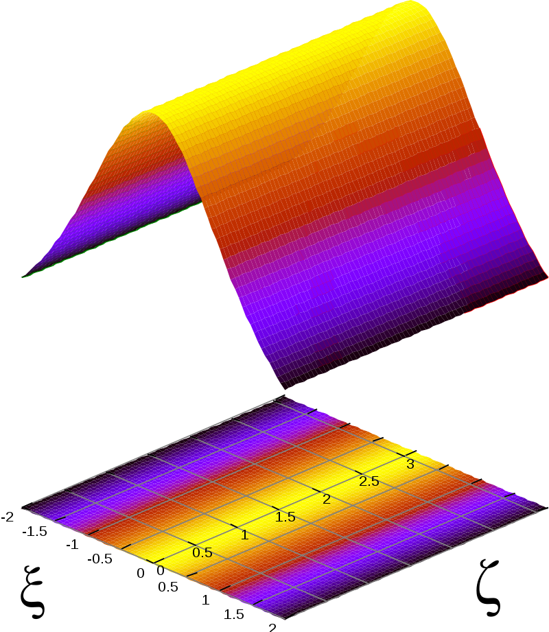
Image: Wikipedia
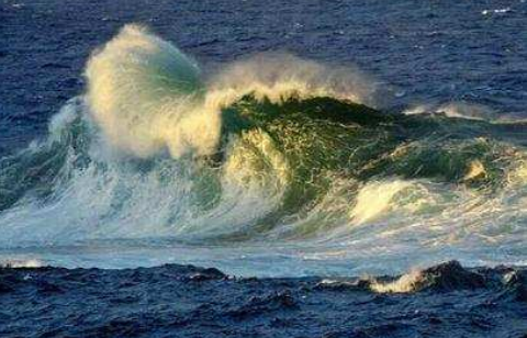
A soliton is a solution of a non-linear partial differential equation, such that
1. Has a permanent form;
2. It is localized within a region;
3. It does not obey the superposition principle;
4. It does not disperse.
For the next few slides, please raise your hand if you think it is a soliton.
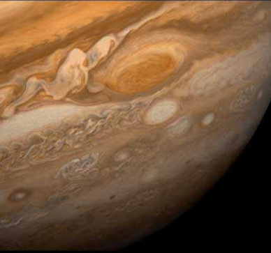
1. Has a permanent form;
2. It is localized within a region;
3. It does not obey the superposition principle;
4. It does not disperse.
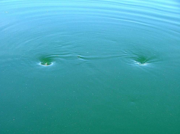
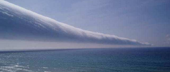
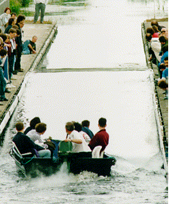
1. Has a permanent form;
2. It is localized within a region;
3. It does not obey the superposition principle;
4. It does not disperse.
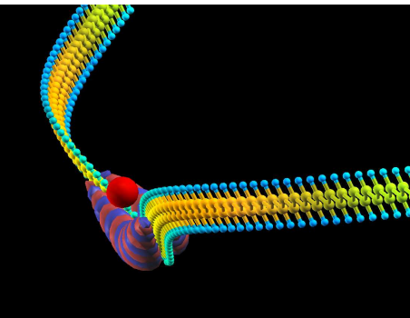
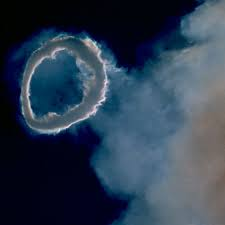
(wavefunction of trans-polyacetylene doped by a counter ion)
kdV equation - Waves
Burgers equation
Nonlinear Schrodinger Equation - Optics
i\partial _{t}\psi =-{1 \over 2}\partial _{x}^{2}\psi +N |\psi |^{2}\psi
{\displaystyle \partial _{t}\phi +\partial _{x}^{3}\phi -6\,\phi \,\partial _{x}\phi =0\,}
{\displaystyle \varphi _{tt}-\varphi _{xx}+\sin \varphi =0,}
Sine-Gordon model - Josephson Junctions
...
Skyrmion model - BEC/Topological solitons
Abrikosov-Nielsen-Olesen model - Superconductivity
i\partial _{t}\psi =-{1 \over 2}\partial _{x}^{2}\psi +N |\psi |^{2}\psi
{\displaystyle \partial _{t}\phi +\partial _{x}^{3}\phi -6\,\phi \,\partial _{x}\phi =0\,}
{\displaystyle \varphi _{tt}-\varphi _{xx}+\sin \varphi =0,}
Dispersive terms in non-linear equation: energy is not conserved
Mathematical property common between all solition solutions: the PDEs are integrable.
Order
within
Chaos
Integrable systems
(solvable)

Fluid dynamics
(complete chaos)

Wave equation (complete order)
more dispersion
no dispersion
Image: Wikipedia
Solitons occur exactly at the regime where the system is non-linear but integrable.
Gaussian pulse in nonlinear media
Gaussian pulse in nonlinear media + third order dispersion
Full playlist: Christophe FINOT
N = 1 solition in nonlinear media
N = 3 soliton in nonlinear media
Full playlist: Christophe FINOT
N = 5 solition in nonlinear media
N = 3 soliton in nonlinear media, + third order dispersion
Full playlist: Christophe FINOT
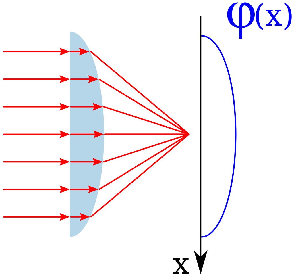
\varphi (x)=k_{0}nL(x)
Phase shift is a function of the geometry
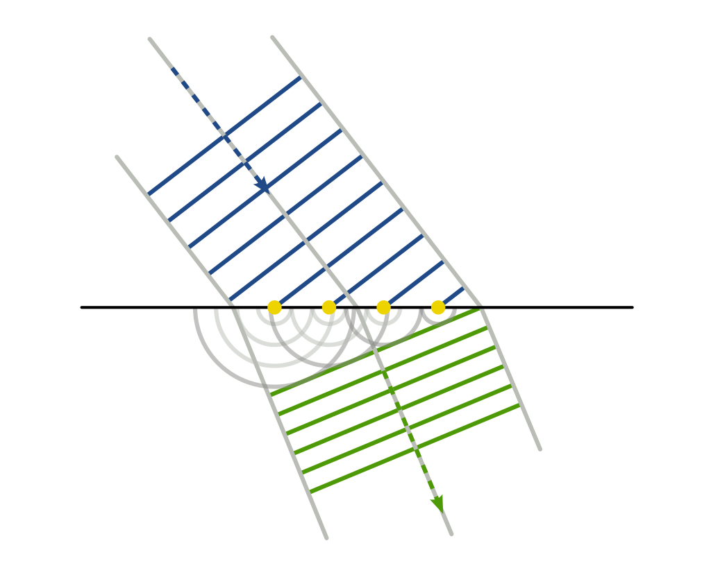
Huygens Fresnel principle
Spatial solitons
Images: Wikipedia
\varphi (x)=k_{0}nL(x)
Phase shift is a function of the geometry
\varphi (x)=k_{0}n(x)L=k_{0}L[n+n_{2}I(x)]
If we had an intensity distribution that had the same amount of phase shift, we get a self-focusing effect while removing the \(x\) dependence from \(L\).
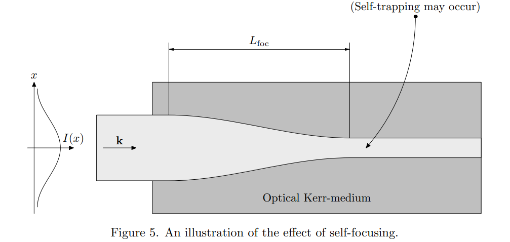
Self-focusing: main mechanism to generate squeezed light
Image: http://jonsson.eu/research/lectures/lect10/lect10.pdf
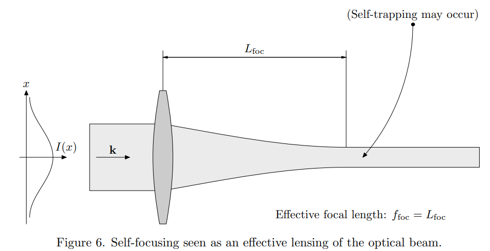
Image: http://jonsson.eu/research/lectures/lect10/lect10.pdf
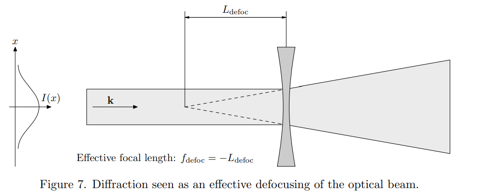
Image: http://jonsson.eu/research/lectures/lect10/lect10.pdf
Kerr effect
n = n_0 + n_2 I
When the refractive index \(n\) is proportional to the intensity of the wave.
Two types of solitons:
- Spatial solitons
- Temporal solitons
n = n_0 + n_2 I(x)
n = n_0 + n_2 I(t)
Proof sketch. Let \(n(I)\) be the refractive index as a function of intensity.
n(I)=n+n_{2}I(x)
Equation of non-linear media
\mathbf{E}(x,z,t)=a_x(z)e^{{i(k_{0}n(I)z-\omega t)}}
\nabla ^{2}\mathbf{E}+k_{0}^{2}n^{2}(I)\mathbf{E}=0
The electric field inside
Helmholtz equation
Derivation of NLSE
\mathbf{E}(x,z,t)=a_x(z)e^{{i(k_{0}n(I)z-\omega t)}}
\nabla ^{2}\mathbf{E}+k_{0}^{2}n^{2}(I)\mathbf{E}=0
The electric field inside
Helmholtz equation
{\displaystyle \left|{\frac {\partial ^{2}a_x(z)}{\partial z^{2}}}\right|\ll \left|k_{0}{\frac {\partial a_x(z)}{\partial z}}\right|}
Assuming the amplitude changes slowly respect to \(z\)
{\displaystyle {\frac {\partial ^{2}a_x}{\partial x^{2}}}+i2k_{0}n{\frac {\partial a_x}{\partial z}}+k_{0}^{2}\left[n^{2}(I)-n^{2}\right]a_x=0.}
Obtain.
{\displaystyle {\frac {\partial ^{2}a_x}{\partial x^{2}}}+i2k_{0}n{\frac {\partial a_x}{\partial z}}+k_{0}^{2}\left[n^{2}(I)-n^{2}\right]a_x=0.}
{\displaystyle \left[n^{2}(I)-n^{2}\right]=[n(I)-n][n(I)+n]=n_{2}I(2n+n_{2}I)\approx 2nn_{2}I}
Drop terms with \(I^2\)
{\displaystyle {\frac {1}{2k_{0}n}}{\frac {\partial ^{2}a}{\partial x^{2}}}+i{\frac {\partial a}{\partial z}}+{\frac {k_{0}nn_{2}}{2\eta _{0}}}|a|^{2}a=0}
Non linear schrodinger equation
{\displaystyle {\frac {1}{2k_{0}n}}{\frac {\partial ^{2}a}{\partial x^{2}}}+i{\frac {\partial a}{\partial z}}+{\frac {k_{0}nn_{2}}{2\eta _{0}}}|a|^{2}a=0}
Non Linear Schrodinger equation
(normalized)
\displaystyle{\frac {1}{2}}{\frac {\partial ^{2}a}{\partial \xi ^{2}}}+i{\frac {\partial a}{\partial \zeta }}+N^{2}|a|^{2}a=0
\(N \ll 1\) : Linear terms dominate
\(N \gg 1\): Non linear part dominates
For soliton solutions, \(N\) must be an integer, called the order of the soliton.
\displaystyle{\frac {1}{2}}{\frac {\partial ^{2}a}{\partial \xi ^{2}}}+i{\frac {\partial a}{\partial \zeta }}+N^{2}|a|^{2}a=0
{\displaystyle a(\xi ,\zeta )=\operatorname {sech} (\xi )e^{i\zeta /2}}
{\displaystyle a(\xi ,\zeta )={\frac {4[\cosh(3\xi )+3e^{4i\zeta }\cosh(\xi )]e^{i\zeta /2}}{\cosh(4\xi )+4\cosh(2\xi )+3\cos(4\zeta )}}.}
\( N\) = 1
\( N\) = 2
Solutions to NLSE
{\displaystyle a(\xi ,\zeta )=\operatorname {sech} (\xi )e^{i\zeta /2}}
{\displaystyle a(\xi ,\zeta )={\frac {4[\cosh(3\xi )+3e^{4i\zeta }\cosh(\xi )]e^{i\zeta /2}}{\cosh(4\xi )+4\cosh(2\xi )+3\cos(4\zeta )}}.}
\( N\) = 1

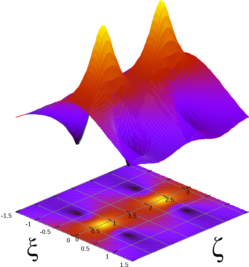
\( N\) = 2
Image: Wikipedia

Image: Wikipedia
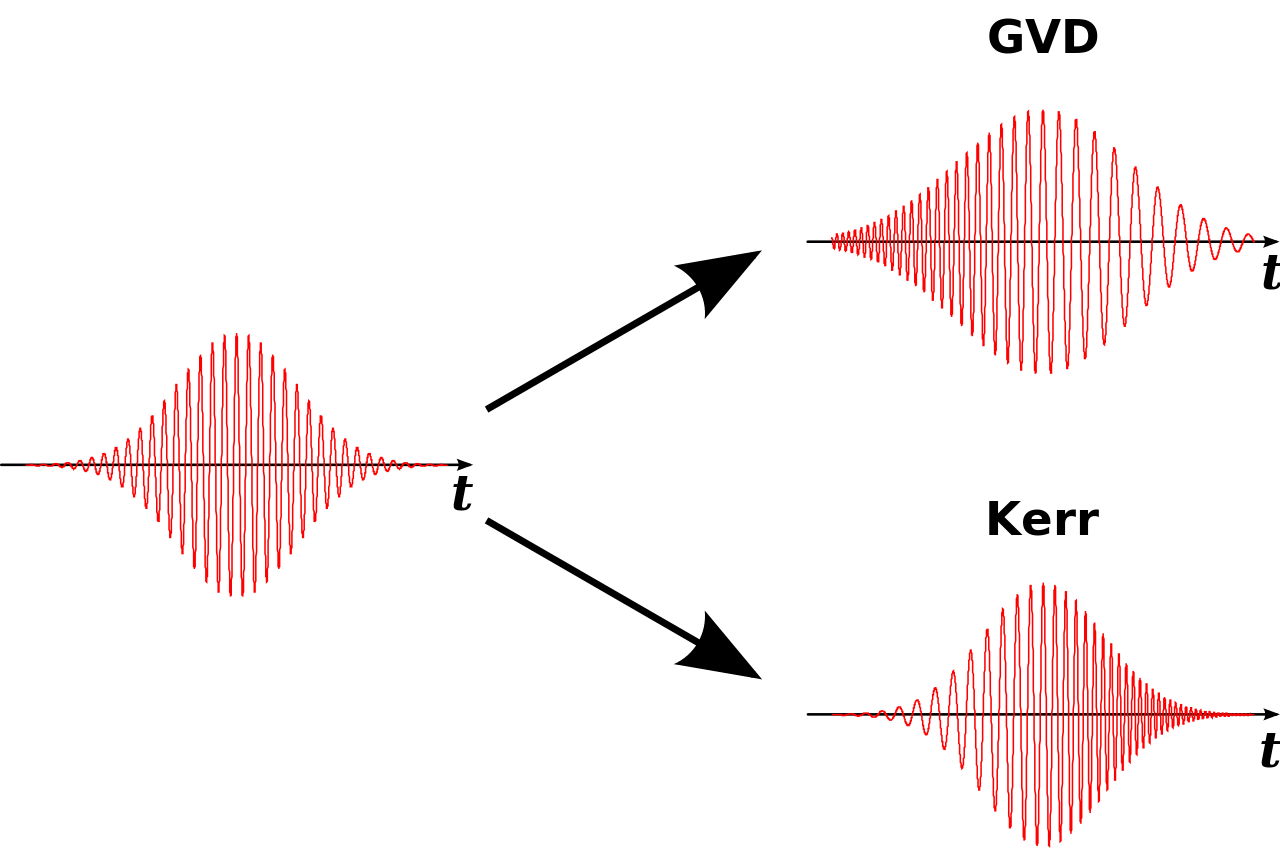
Dispersion
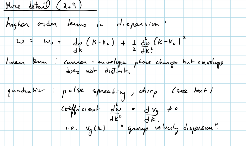
Group velocity Dispersion
Non-linear dispersion relation implies \(v_g \neq v_p \)
{\displaystyle D=\frac{d^2\omega}{dk^2} = \frac{dv_g}{dk}}

Image: Wikipedia
\(D > 0\): anomalous dispersion. \(k = \omega^2 \)
-
higher frequency arrives faster/[slower] than lower frequency
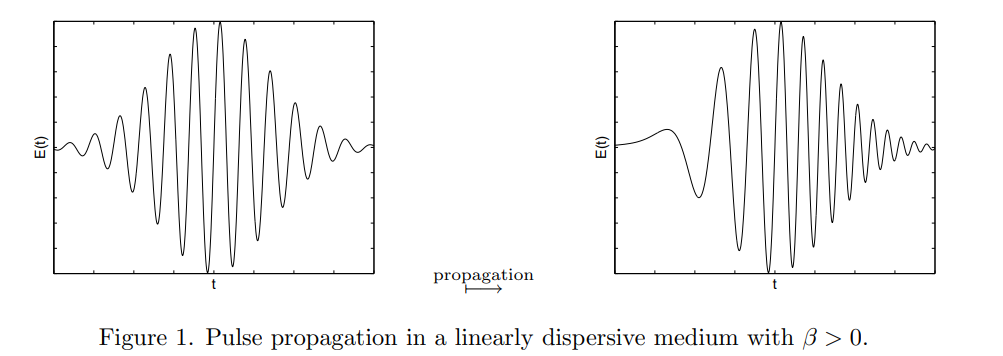
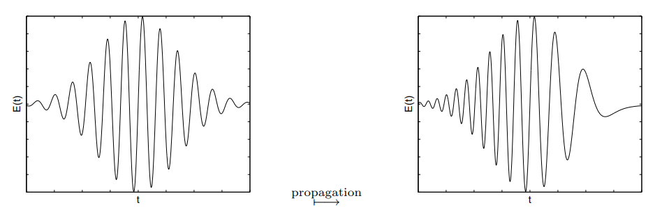
D < 0: normal dispersion
D > 0: anomalous dispersion
Image: http://jonsson.eu/research/lectures/lect10/lect10.pdf
Temporal solitons
\varphi (t)=\omega _{0}t-k_{0}z[n+n_{2}I(t)]
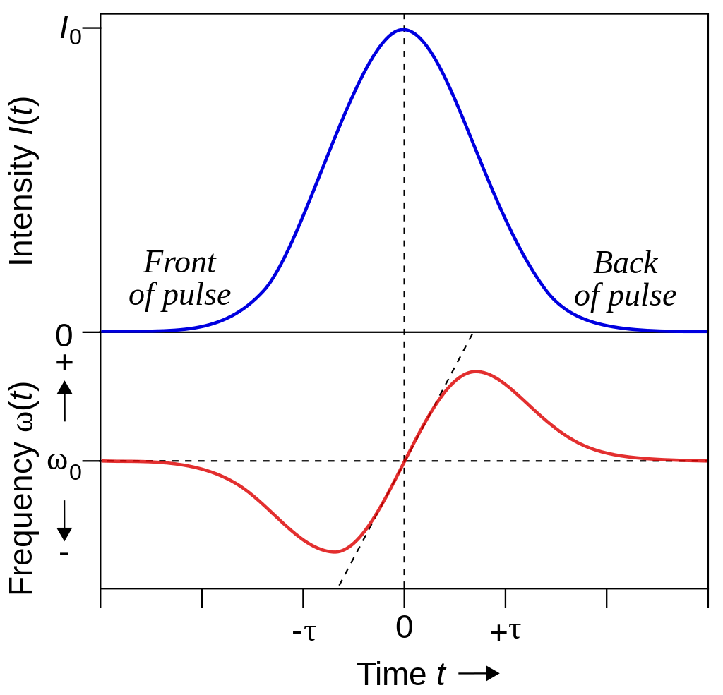
\omega (t)={\frac {\partial \varphi (t)}{\partial t}}=\omega _{0}-k_{0}zn_{2}{\frac {\partial I(t)}{\partial t}}
Image: Wikipedia
Temporal solitons
D > 0
anomalous dispersion
Kerr effect: self focusing
Image: Wikipedia
PDE for temporal solitons still the NLSE: Proof on Wikipedia
{\frac {1}{2}}{\frac {\partial ^{2}a}{\partial \tau ^{2}}}+i{\frac {\partial a}{\partial \zeta }}+N^{2}|a|^{2}a=0
The derivation is the exact same except now we need to derive the equation in frequency domain, Fourier transform back.
So far, we have assumed:
- \(D > 0\) (temporal solitons) or
- \(n_2 > 0\) (spatial solitons)
What if \(D < 0\) or \(n_2 < 0\)?
Temporal solitons: \(D > 0\)
D > 0
anomalous dispersion
Kerr effect: self focusing
Kerr
GVD
What if \(D < 0\) or \(n_2 < 0\)?
Temporal solitons: \(D < 0\)
D < 0
Normal dispersion
Kerr effect: self focusing
Kerr
GVD
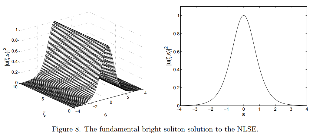
{\displaystyle a(\xi ,\zeta )=\operatorname {sech} (\xi )e^{i\zeta /2}}
\(D > 0\) or \(n_2 > 0\)
Image: http://jonsson.eu/research/lectures/lect10/lect10.pdf
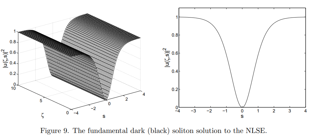
a(\xi, \zeta)=a_0 \tanh \left(a_0 \xi \right) \exp \left(i a_0^2 \zeta\right)
\(D < 0\) or \(n_2 < 0\)
Image: http://jonsson.eu/research/lectures/lect10/lect10.pdf
Timeline of solitons
-
-
1974: Spatial solitons first discovered [4]
-
1987: Experimental observation of dark solitons [11]
-
- Kerr effect
- Spatial solitons: counters diffraction
- Temporal solitons: counters dispersion
- Bright solitons
- Dark solitons
- How to get squeezed light
i\partial _{t}\psi =-{1 \over 2}\partial _{x}^{2}\psi +N |\psi |^{2}\psi
\psi(x) = N \textrm{sech}(x)
NLSE
Fundamental solition \(N = 1\)
Image: Wikipedia
Main References
[1] A. Hasegawa and F. Tappert, Transmission of Stationary Nonlinear Optical Pulses in Dispersive Dielectric Fibers. I. Anomalous Dispersion, Appl. Phys. Lett. 23, 142 (1973).
[2] A. Hasegawa and F. Tappert, Transmission of Stationary Nonlinear Optical Pulses in Dispersive Dielectric Fibers. II. Normal Dispersion, Appl. Phys. Lett. 23, 171 (1973).
[3] Y. Song, X. Shi, C. Wu, D. Tang, and H. Zhang, Recent Progress of Study on Optical Solitons in Fiber Lasers, Applied Physics Reviews 6, 021313 (2019).
[4] J. E. Bjorkholm and A. A. Ashkin, Cw Self-Focusing and Self-Trapping of Light in Sodium Vapor, Phys. Rev. Lett. 32, 129 (1974).
[5] G. I. Stegeman and M. Segev, Optical Spatial Solitons and Their Interactions: Universality and Diversity, Science 286
[6] F. Jonsson, Lecture Notes on Nonlinear Optics (2003). http://jonsson.eu/research/lectures/
The Elements of Nonlinear Optics (Cambridge University Press, Cambridge, 1990).
References
[8] Y. S. Kivshar, Optical Solitons: From Fibers to Photonic Crystals / Yuri S. Kivshar, Govind P. Agrawal. (Academic Press, 2003).
[9] P. G. Drazin and R. S. Johnson, Solitons: An Introduction, 2nd ed. (Cambridge University Press, Cambridge, 1989).
[10] J. K. Shaw, Mathematical Principles of Optical Fiber Communications / J.K. Shaw. (Society for Industrial and Applied Mathematics, 2004).
[11] P. Emplit, J. P. Hamaide, F. Reynaud, C. Froehly, and A. Barthelemy, Picosecond Steps and Dark Pulses through Nonlinear Single Mode Fibers, Optics Communications 62, 374 (1987).
[12] K. Ikeda, K. Suzuki, R. Konoike, S. Namiki, and H. Kawashima, Large-Scale Silicon Photonics Switch Based on 45-Nm CMOS Technology, Optics Communications 466, 125677 (2020).
Optical Solitons
By Zhi Han


