Overview of

Abstraction-Based Parameter Synthesis

for Multiaffine Systems

Alexander Bykovsky

email: control.eight@gmail.com

 Hybrid automata

Hybrid systems combine continuous and discrete dynamics interaction. Somehow we need to capture dynamics of the continuous parts of the system with the dynamics of the logic and discrete parts.

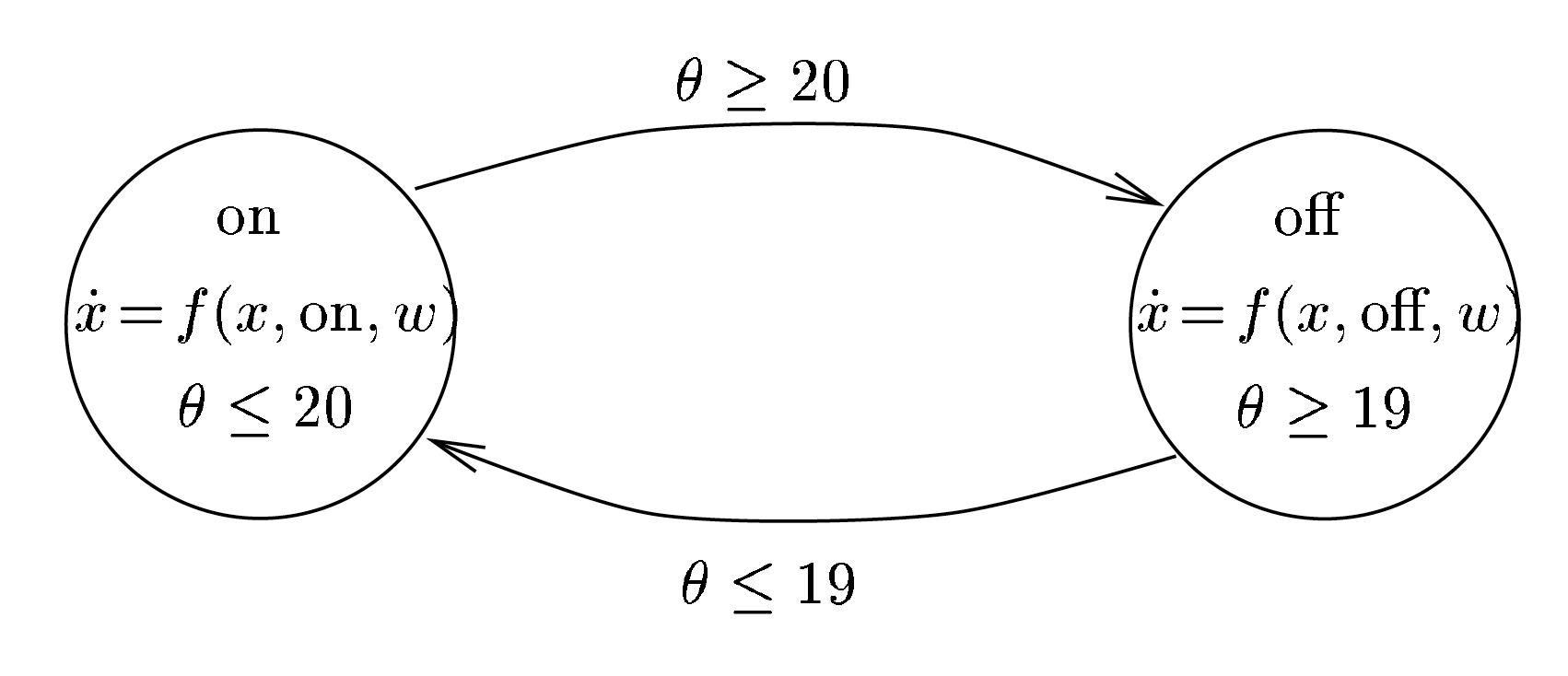
Temperature-thermostat system as a hybrid automation

A hybrid automaton (HA) is a mathematical model with

both continuous and discrete behavior. It is represented by the tuple H = (Loc, Var, Inv, Flow, Trans, Init ).

Loc is a set of discrete locations.

Var is a set of real-valued variables x1, . . . , xn.

Flow (ℓ ) is a set of differential equations (or inclusions) that defines the time-driven evolution of the continuous variables.

The set of discrete transitions Trans defines how the state can jump between locations when inside the transition’s guard set.

The system can remain in a location ℓ while the state is inside the

invariant set Inv (ℓ ). 

All behavior originates from the set of initial states Init .

A state s ∈ Loc x R^n consists of a location and values

of the continuous variables x1, . . . , xn .

Temperature-thermostat system as a hybrid automation formal description

Loc ∈ {on, off}

Var ∈ [~18, ~21]

Flow ∈ {x ̇ =−a(x−b),x ̇ =−ax}, a > 0, b >= 20 - some temprature towards what it increases    

Trans ∈ {(on, >= 20), (off, <= 19)}

Init ∈ {(on, 19.5),(on, 18.5), (off, 19.5), (off, 20.01)}

Inv ∈ {<= 20, >= 19}

States ∈ {(on, 18.67), (on, 19.5), (off, 20.1), (off, 19.5}

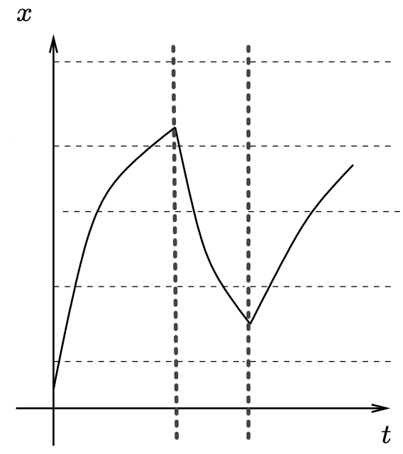
 A possible trajectory of the thermostat system

18.5

19

20

19.5

On

Off

On

20.5

Verification problems

In the verification setting, we are interested in whether there exists a trajectory from the set Init to a set Bad which defines the bad states to be avoided.

Two central problems in formal analysis are reachability analysis and safety verification.

Convex approximation technique

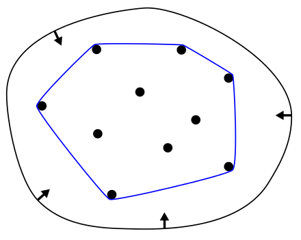
There is as stepwise refinement design method in which one starts of an abstract level that allows relatively easy verification, and then processes in steps to more and more refined deisgns. Then complicated description of a part of the system is replaced by some coarse information. This process is sometimes called abstraction.

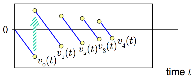
Bouncing Ball Example

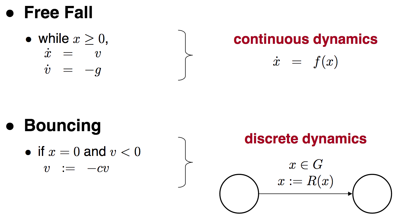
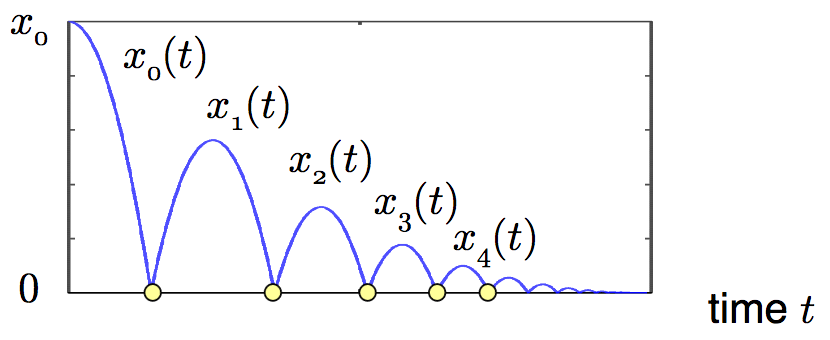
Position / time

Velocity / time

Reachability analysis

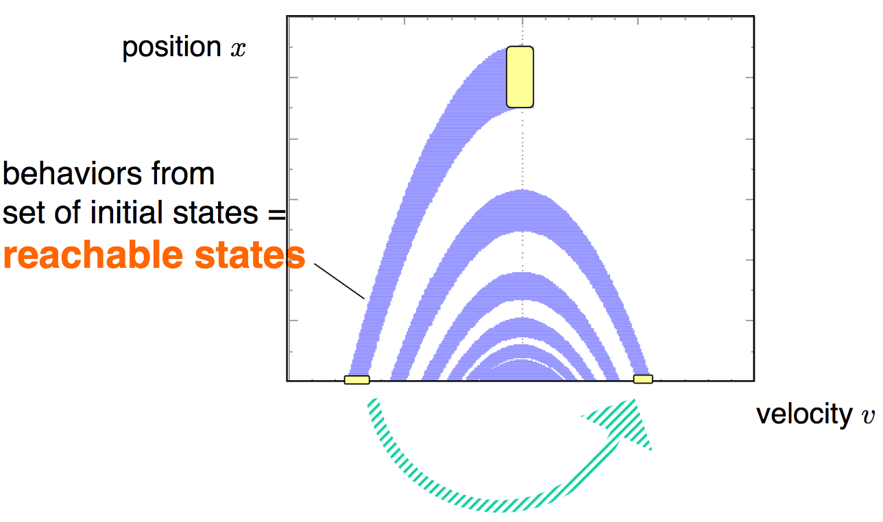
State-space consists of: position and velocity

We need to decide if there exists a trajectory of the hybrid system that reaches a given set of states.

Parameter synthesis problem which is to identify sets of parameters for which the system does (or does not) reach a given set of states. The term “parameter” refers to both the initial conditions of the model (e.g., thermostat is switched on at time t = 0) and dynamical parameters (e.g., temperature has specific value).

Parameter synthesis

For example, in the context of a thermostat and an air conditioner, we might be interested in partitioning the parameter space into two regions — those that, with heating is switched on, deterministically lead to the an air conditioner working properly, and those that lead to an air conditioner to be broken.

The parameter synthesis problem is relatively easy to solve when the system has linear dynamics, and there are a variety of methods for doing so.

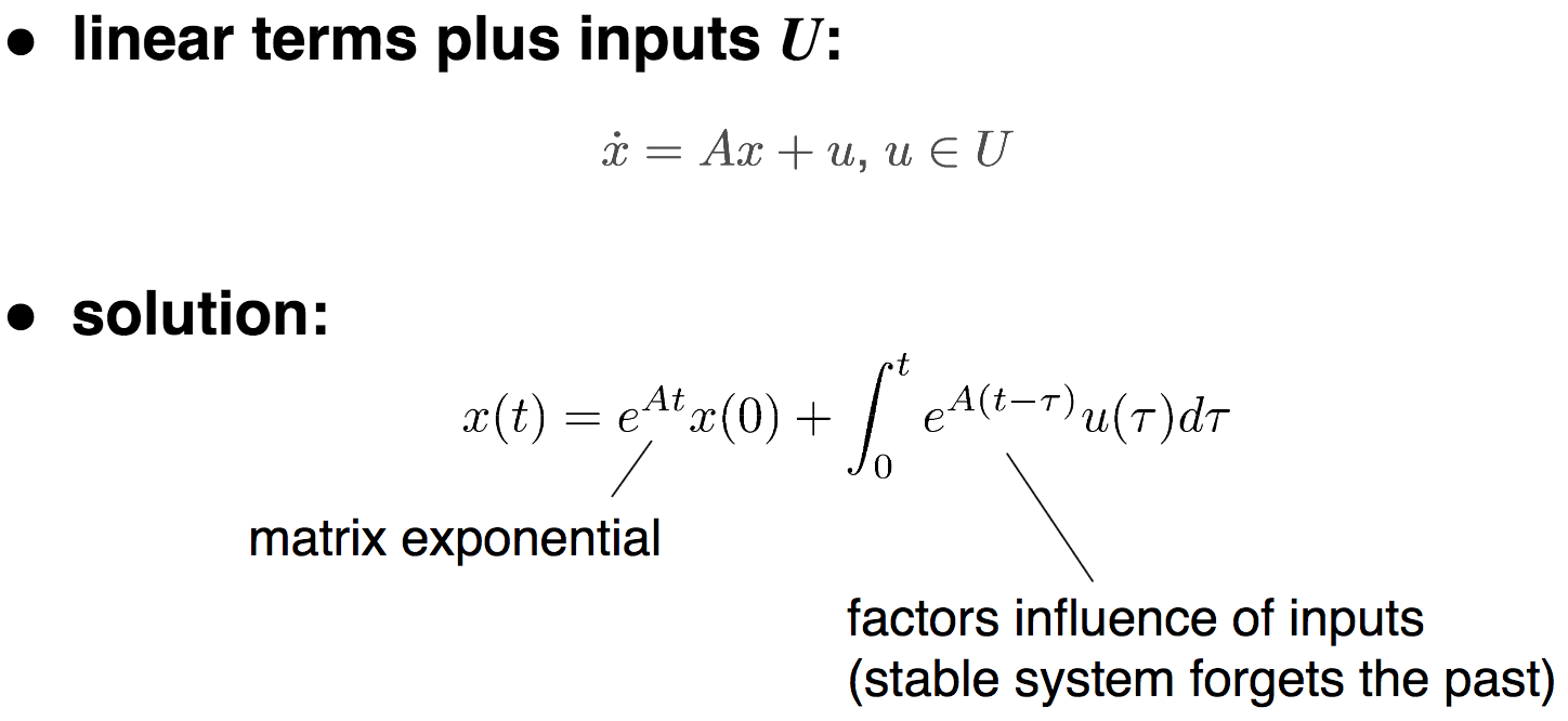
Linear hybrid automata (LHA)

Let x (t) ∈ R^n denote the values of the continuous variables at time t. We consider continuous dynamics Flow of the following two forms. If x˙ (t ) ∈ P where P  is a polytope, then the HA is called a linear hybrid automaton (LHA), considering convex polytopes.

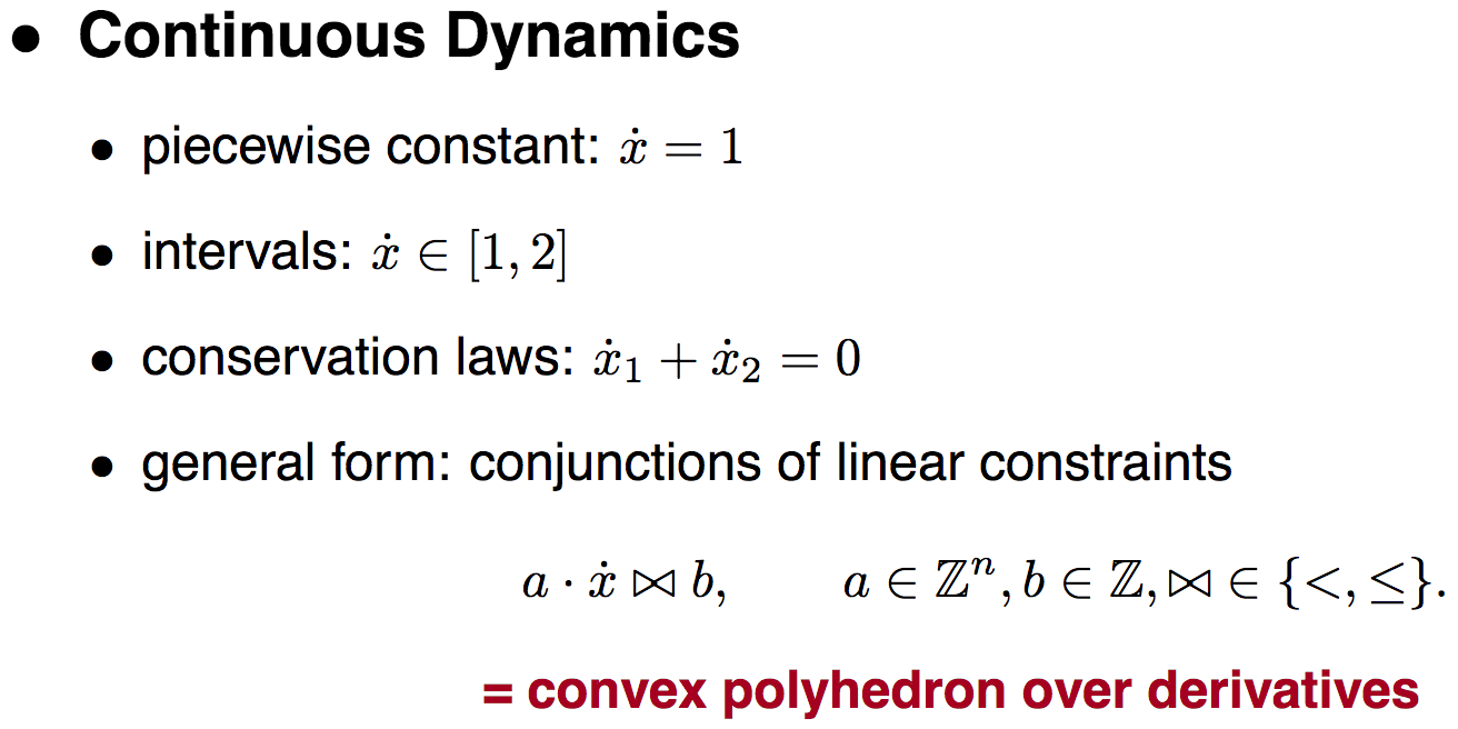
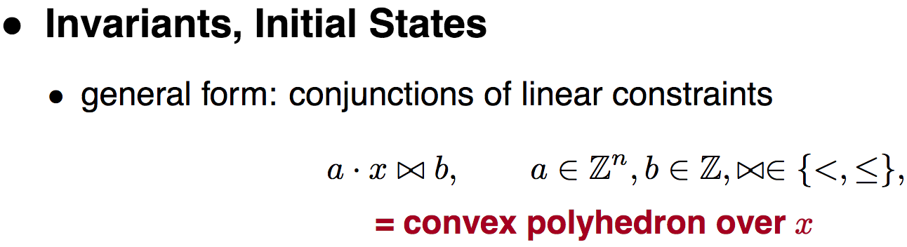
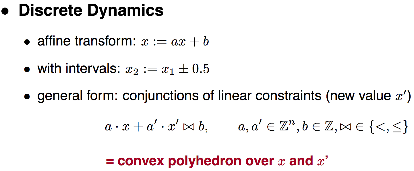
Convex  polyhedron

Genetic regulatory network

is defined by the dynamics of the following form:

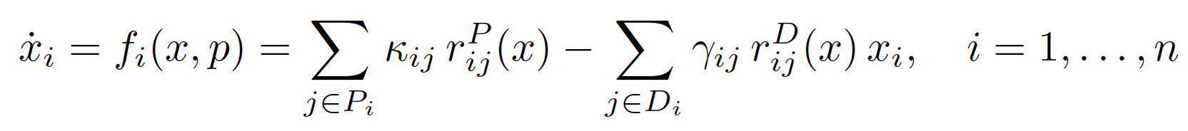
Here xi is the i-th component of the state vector x ∈ X ⊂ R^n . Pi and Di are sets of indices. κij and γij are production and degradation rate parameters, respectively.

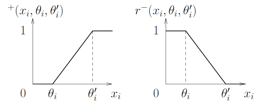
The terms rij are continuous piecewise-multiaffi ne functions arising from products of ramp functions r+ and r−.

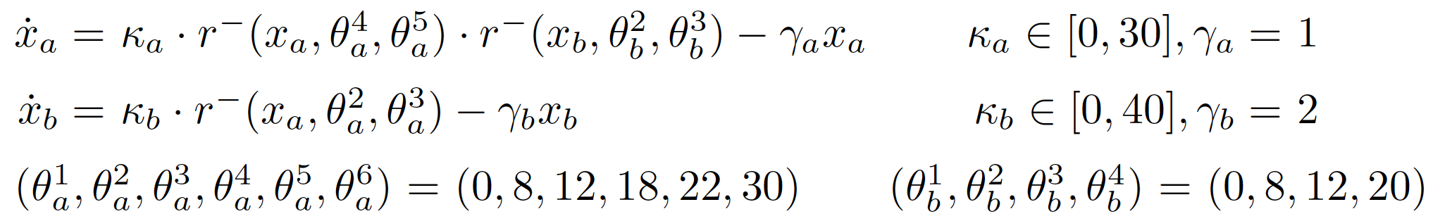
Example (two-genes network):

Affine dynamics

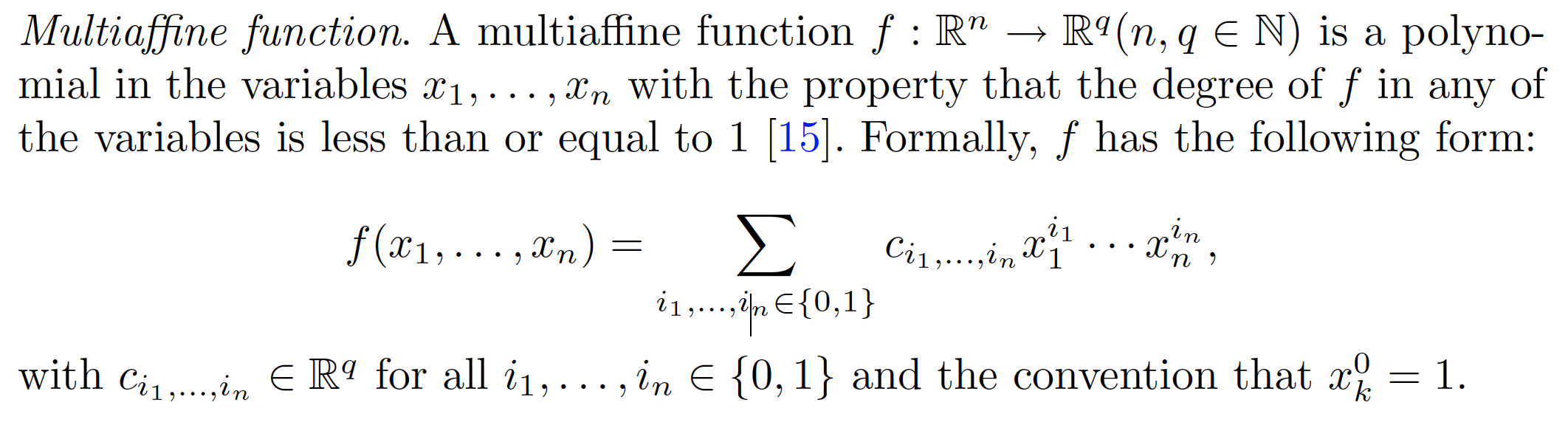
 Multiaffine function

Example (two genes network):

Ramp functions:

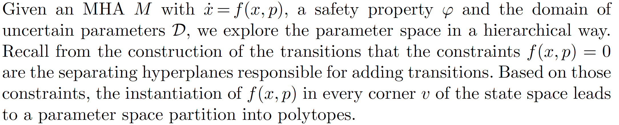
Multiaffine hybrid automata (MHA)

If x˙ (t) = f (x, t) where f (x, t) is a multiaffine function, then the HA is called a multiaffine hybrid automaton  (MHA). It helps to model systems with highly nonlinear behavior​.

It's difficult to solve verification problem for MHA. And we don't have a good solution for this as for LHA like SpaceEx.

In our case f(x, t) = 

Where ka - is - p - uncertain parameter. So our function is multiaffine in x but affine in p. So we can use LHA to explore state space of uncertain parameters - P.

Our goal is to identify a subset of the parameter domain D  which ensures that the property ϕ holds for a given MHA, i.e., RBad is avoided when starting in RInit .

Goal and Solution

We first introduce an LHA Lm (p) which overapproximates the behavior of the transition system TM (p) for a particular parameter value p ∈ D. In particular, we map every hyper-rectangular region to a location in the LHA and use the bounds on the regions as invariants.

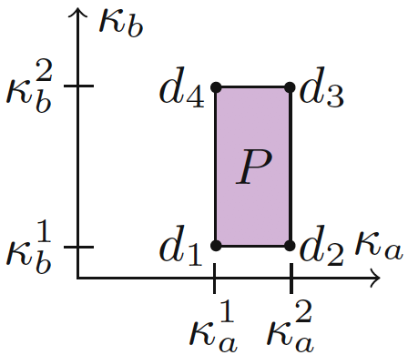
The system is parametrized by the vector p  = (p1, ..., pm ) ∈ D , where D  is the hyper-rectangular domain of uncertain parameters.

Text

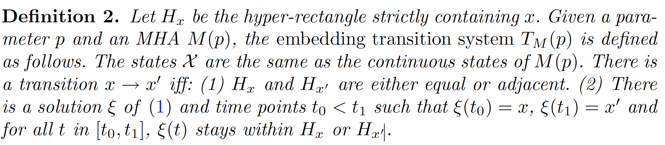
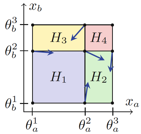
From state space partition to transition system

Example for κa = 10 and

κb = 15 (arrows normalized)

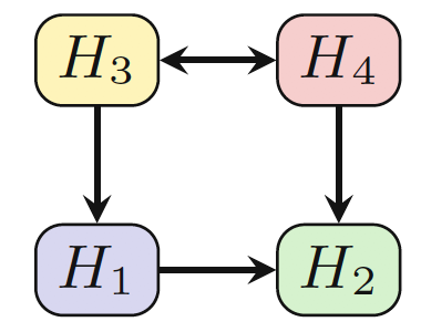
From state space partition to transition system. Modeling with SpaceEx

Let's define H1, H2, H3, H4 for our example where κa = 10 and κb = 15. The most important is to define flows.

Flow for H1:

Flow for H2:

(a)

(b)

(a) and

(c)

Flow for H3:

(d)

and (b)

Flow for H4:

(d) and (c)

From state space partition to transition system. Modeling with SpaceEx

Finally model for H1, H2, H3, H4 using SpaceEx will look like the following. Please note that this is a LHA. It defines Loc (H1, H2, H3, H4), Var (xa, xb), Inv (4 invs), Flow (defined above), Trans (t1, t2, t3, t4, t33). 

One can notice that all Flows are affine.

From state space partition to transition system. Modeling with SpaceEx

Let's check some transitions. Init: xa = 0, xb = 0, init locaiton: H1. Should be transition from H1 to H2.

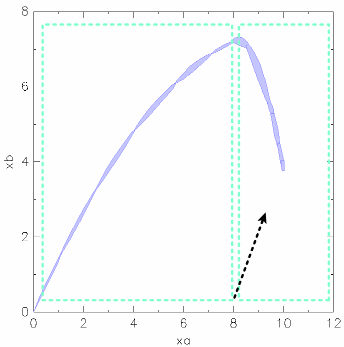
H1

H2

From state space partition to transition system. Modeling with SpaceEx

Init: xa = 8, xb = 4, init location: H2. There shouldn't be any transitions.

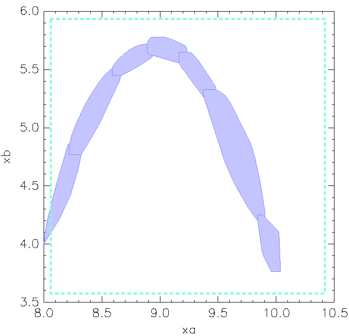
H2

From state space partition to transition system. Modeling with SpaceEx

Init: xa = 10.2, xb = 12, init locaiton: H4. Transitions: H4 -> H3 -> H1 -> H2.

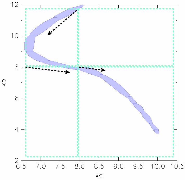
H1

H2

H4

H3

Modeling transition system

LM( p) has a transition from location ℓ to ℓ′ associated with

hyper-rectangles Hℓ and Hℓ′ only if the projection of f( x, p) on the Hℓ→ Hℓ′ direction is positive in at least one corner of the facet separating Hℓ from Hℓ′ .

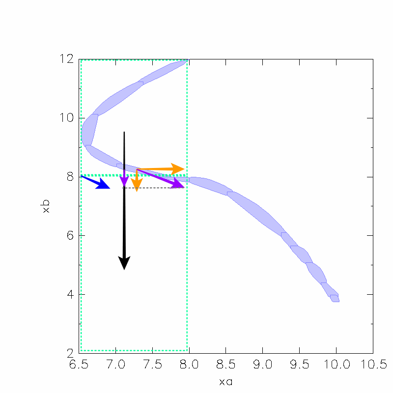
Transition direction

Projection

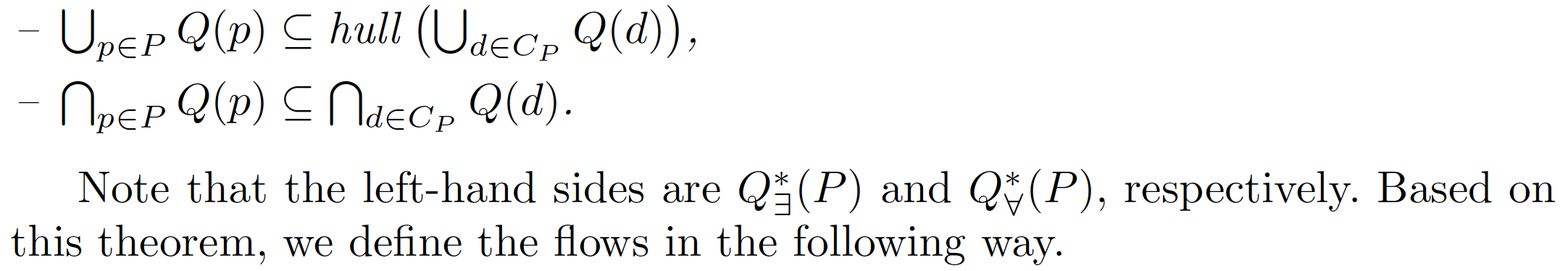
 Set-Based LHA Abstraction

L∃M(P) has a transition from location ℓ to ℓ′ if there is a transition from ℓ to ℓ′ in LM(p) for some p ∈ P. Analogously, LaM(P) has a transition from location ℓ to ℓ′ if there is a transition from ℓ to ℓ′ in LM(p) for all p ∈ P.

For example for our case there is a transition from H1 to H2 for κa = 10 and κb = 15. So we can conclude that L∃M(P) has a transition from location H1 to H2. If we check that all values for ka and kb lead us to a transition from H1 to H2 then we can also conclude that LaM(P) has a transition from location H1 to H2.

 Set-Based LHA Abstraction

Then we define:

For H1 we've got the following state equations:

 Set-Based LHA Abstraction. Example

 Discrete Abstraction of MHA

Clearly, the induced Kripke structure is a conservative abstraction of the LHA as it allows for additional trajectories to the bad states for two reasons. The behavior in the states is unconstrained due

to the absence of flows, and the initial and bad states of the Kripke structure overapproximate their LHA counterparts.

 Parameter Identification

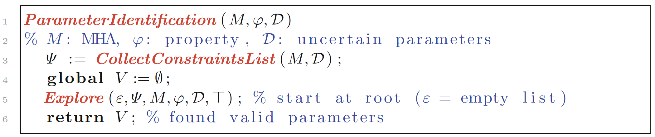
 Parameter Identification

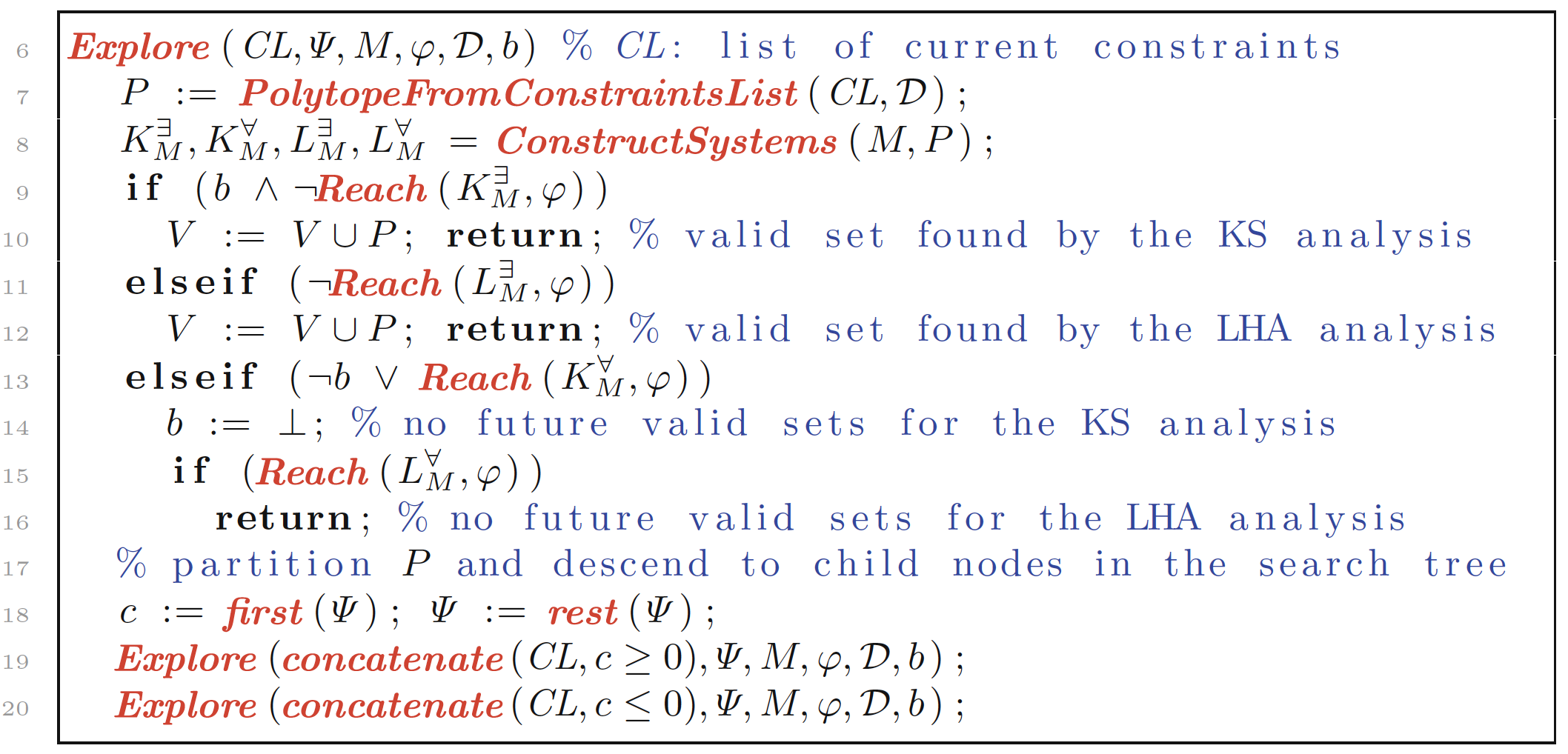
This function takes a list CL  of constraints which encodes hyperplanes used to define the current parameter set.

 Parameter Identification

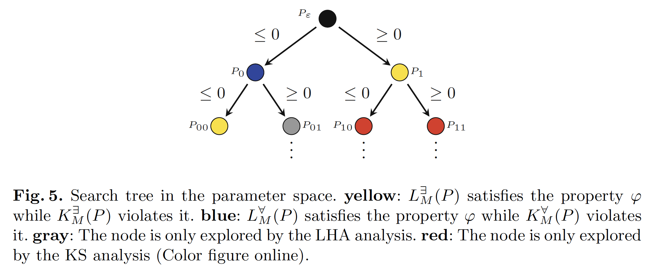
Recursively it will be going as if it's a binary tree. So from algorithmic complexity analysis prospective there will be O(2^n) computations.

Evaluation

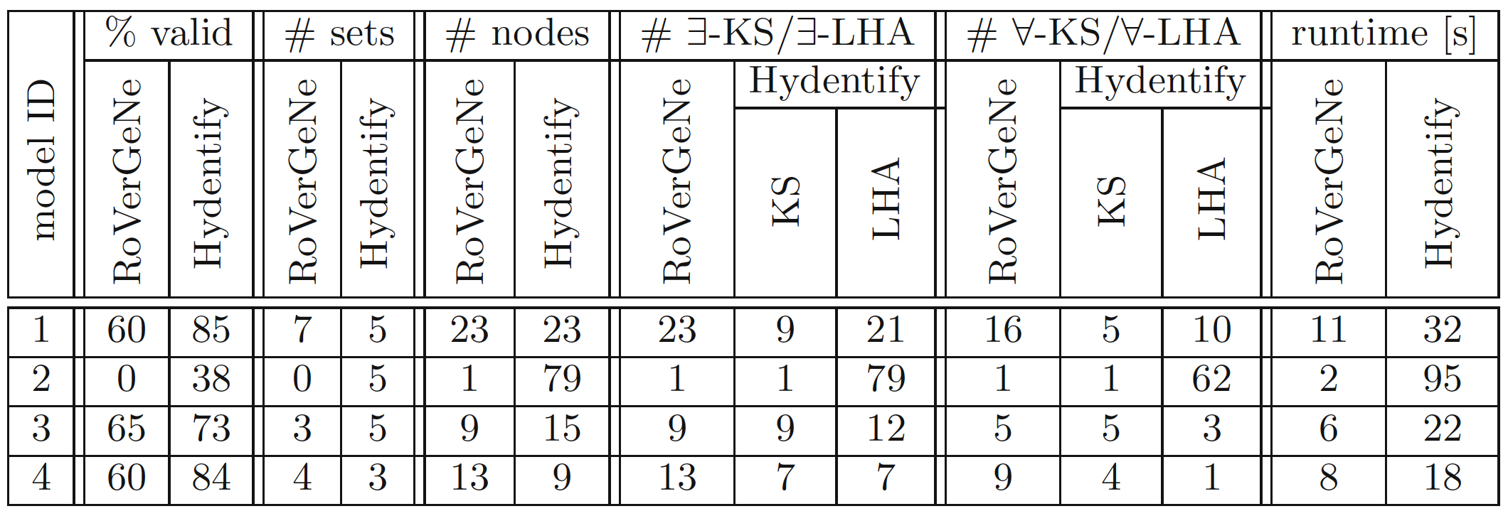
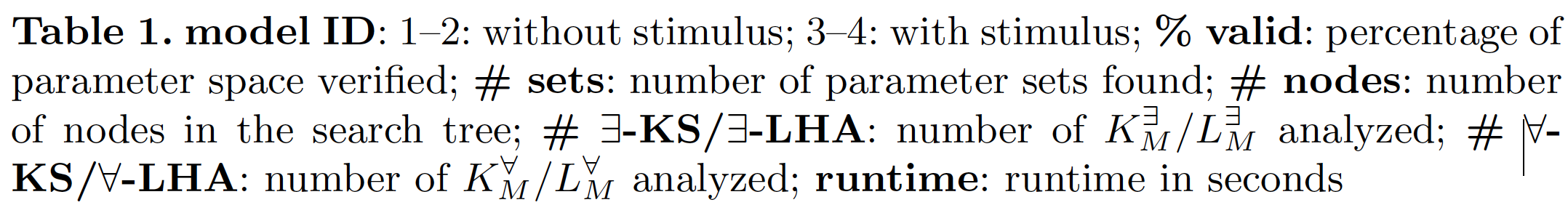
Evaluation

To summarize there are following advantages:

1. This model tends to have better parameter coverage
2. This model can identify more sets with valid parameters
3. It shrinks a space in much precise way (more nodes in a search tree)
4. This model treats time as a continuous  entity.
5. Acceptable runtime execution time.
6. Employing the symbolic model and using LHA allow us to use existing state of the art tools such as SpaceEx.

7. This approach has a large potential with respect to parallelization.

Conclusion

Given a parameter polytope P, we compute an LHA which overapproximates the system behavior for P. Furthermore, we compute another LHA which enables us to prune the search tree. We have evaluated our approach on a model of a genetic regulatory network and a myocyte model and demonstrated its improvement over RoVerGeNe, a tool for parameter identification based on a purely discrete abstraction.