


Alexander W. Winkler
Robotics researcher specialized in motion planning for legged systems.
Alexander W. Winkler, Dario Bellicoso, Marco Hutter, Jonas Buchli
Paper published in IEEE Robotic and Automation Letters (RA-L 2018) \( \cdot \) DOI: 10.1109/LRA.2018.2798285
\( \bullet \) traverse rubble in earthquake \( \bullet \) reach trapped humans \( \bullet \) climb stairs \( \bullet \)...
Agility ...vs rolling
Strength ...vs flying
\( \bullet \) carry heavy payload \( \bullet \) open heavy doors \( \bullet \) rescue humans \( \bullet \) ...
vs
Source:
ANYbotics, Anymal bear, "Image: https://www.anybotics.com/anymal", 2018; Boston Dynamics, Atlas, "Image: https://www.bostondynamics.com/atlas", 2016; Italian Institute of Technology, HyQ2Max "Image: https://dls.iit.it/robots/hyq2max, 2018; Alphabet Waymo, Firefly car, "Image: https://waymo.com", 2016, DJI, Phantom 2 drone, "Image: https://www.dji.com/phantom-2", 2016
Source: https://www.youtube.com/watch?v=NX7QNWEGcNIa
Source: https://www.youtube.com/watch?v=arCOVKxGy9E
Goal \( \cdot \) position \( \cdot \) velocity \( \cdot \) duration \( \cdot \)
Robot \( \cdot \) kinematic \( \cdot \) dynamic
Environment \( \cdot \) terrain \( \cdot \) friction \( \cdot \) ...
Desired Motion-Plan
Actuator Commands
force \( \cdot \) torque
Tracking
Controller
off-the-shelf
NLP Solver
Mathematical Optimization Problem
Direct Method
Collocation
Task
Gait and Trajectory Optimization for Legged Systems through Phase-based End-Effector Parameterization
IEEE Robotic and Automation Letters (RA-L) \( \cdot \) 2018
A. W. Winkler, D. Bellicoso, M. Hutter, J. Buchli
Mathematical Optimization Problem
predefined / "factorized":
restrict search space
all motion-plans \( \{ \mathbf{x}(t), \mathbf{u}(t) \} \)
fullfills all contraints
keeping search-space as open as possible
Single Rigid Body \( \cdot \) Newton-Euler Equations
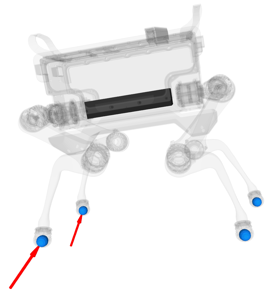
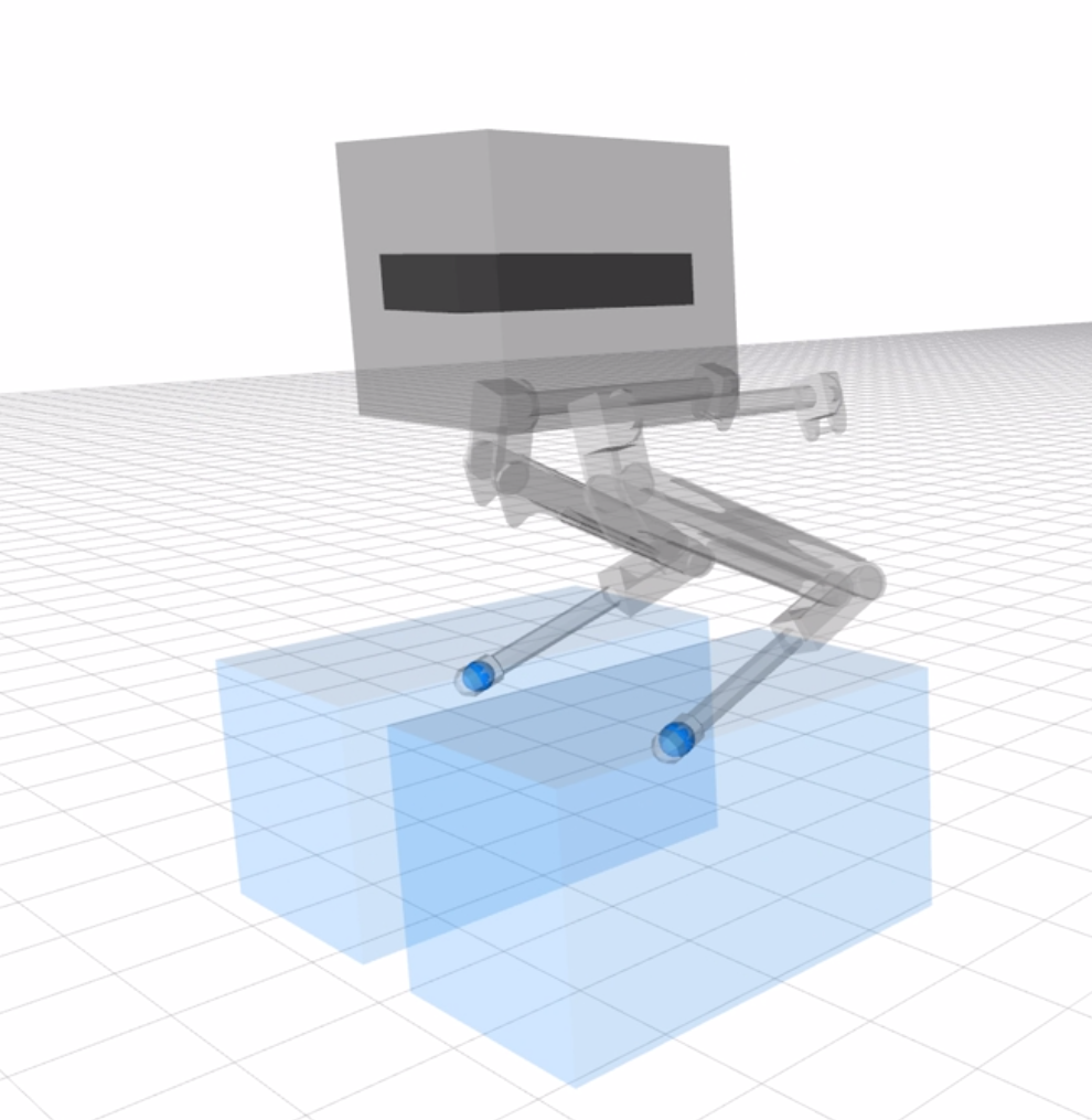
Range-of-Motion Box \(\approx\) Joint limits
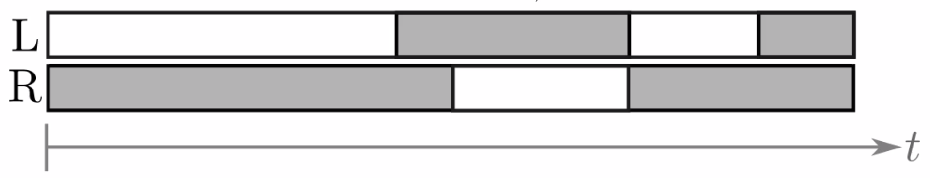
R | 2 | L | R | 2
R | 0 | R | 2 | R | 2
.... gait defined by continuous phase-durations \(\Delta T_i\)
without Integer Programming
Sequence:
swing
stance
individual foot always alternates between and
Phase-Based End-Effector Parameterization
Know if polynomial belongs to swing or stance phase
Foot \( \mathbf{p}_i(t)\) cannot move while
Physical Restrictions
standing
swinging
Foot can only stand on terrain
Forces can only push
Forces inside friction pyramid
Given:
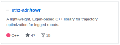
open-sourced software
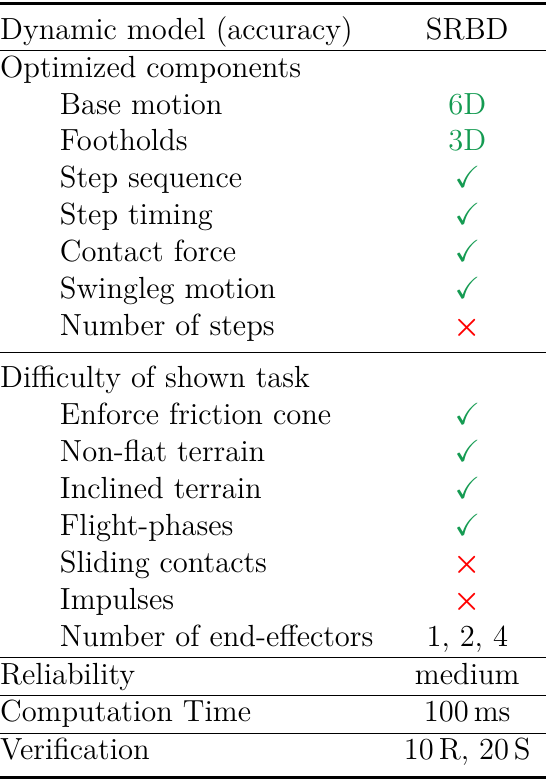
Computation Time 100 ms
1s-horizon, 4-footstep motion for a quadruped
$ sudo apt-get install ros-kinetic-xppThese slides, papers and more at
J. Buchli
M. Hutter
D. Bellicoso
$ sudo apt-get install ros-kinetic-towr_ros$ sudo apt-get install ros-kinetic-ifoptA. Winkler
By Alexander W. Winkler
Paper: https://ieeexplore.ieee.org/document/8283570/ Recorded talk: https://youtu.be/KhWuLvb934g


