Behavioral Incentive Compatibility
David Danz
Lise Vesterlund
Alistair Wilson
Exeter, April 2023
Incentive Compatible Mechanisms
How should we pay?
- Ask
- Ask + Pay
- Ask + Pay + Incentive compatible
Experimental economists are often faced with a choice over how to elicit information
Incentive Compatibility
- For each type there is a different uniquely maximizing choice within the mechanism
- This yields fully separating behavior
- Given this one-to-one correspondence, the analyst can interpret the relevant choice as the type
- Elicitation mechanisms are at the sharp end of mechanism design, using the above correspondence for measurement
- Often as an input into inferential regressions
- Subjective beliefs are a clear example, and are often central for inference
Behavioral Incentive Compatibility
- Need to examine the extent to which the theoretical assumptions holds
- Show that a prominent mechanism with relatively weak theoretic conditions for IC is not behaviorally incentive compatible
- Demonstrate the substantive effects of this failure over: Objective probabilities, Objective posteriors, Subjective beliefs
- Use this to motivate two methodological checks to assess Behavioral Incentive Compatibility
Subjective Beliefs
Manski:
The difficulty is that observed choice behavior may be consistent with many alternative specifications of preferences and expectations…I have concluded that econometric analysis of decision making with partial information cannot prosper on choice data alone… The data I have in mind are self-reports of expectations elicited in the form called for by modern economic theory; that is, subjective probabilities.
Subjective beliefs often central for inference ─ how do we elicit them?
Example of Beliefs in Inference:
Niederle & Vesterlund (QJE 2006)
Main Idea:
Paper examines gender & competition:
- Do women compete less than men?
- Use a clever experimental design to examine tournament entry
- Measure beliefs with a very simple elicitation.
Example of Beliefs in Inference:
Niederle & Vesterlund (QJE 2006)
Use of Beliefs:
Use beliefs in two ways:
- As a left-hand-side variable to examine confidence differences between men and women
- As a right-hand-side variable to assess the degree that confidence differences explain gender differences in competition choices
Evolution of Belief Elicitation
- Niederle & Vesterlund used a very simple (and coarse) elicitation device:
- Modal rank in tournament (paying $1 if correct)
- But the literature has increasingly focused on elicitations of arbitrarily precise probabilities
- Initial IC elicitations assumed risk-neutral EU maximizers: Quadratic Scoring Rule (QSR)
- But risk aversion pushes beliefs to center
- One response to this was to control for risk preferences within the elicitation
- Another was to use an elicitation that is IC for a wider set of preferences
-
Houssain & Okui (2013): the Binarized Scoring Rule
-
Belief elicitation in practice:
-
Incentive compatibly. QSR (Brier, 1950), BSR (Roth and Malouf, 1979; Grether, 1980; Allen, 1987; Hossain and Okui, 2013; Schlag and van der Weele, 2013), BDM (Holt and Smith, 2009; Karni, 2009)
-
Surveys (Manski, 2004; Schotter and Trevino, 2014; Schlag et al., 2015)
-
Distortions and corrections (Offerman et al., 2009, Andersen et al., 2013; Harrison et al., 2013; Armantier and Treich, 2013; Schlag and van der Weele, 2013)
-
Stakes and hedging (Blanco et al., 2010; Coutts, 2019)
-
Does elicitation change behavior? (Croson, 2000; Wilcox and Feltovich, 2000; Rutstrom and Wilcox, 2009; Gächter and Renner, 2010)
Belief elicitation in practice:
- Does incentivization matter? (Offerman and Sonnemans, 2004; Gächter and Renner, 2010; Wang, 2011; Trautmann and van de Kuilen, 2014)
-
Does properness matter? (Nelson and Bessler, 1989; Palfrey and Wang, 2009)
-
Consistency with actions (Cheung and Friedman, 1995; Nyarko and Schotter, 2001; Costa-Gomes and Weizsäcker, 2008; Rey-Biel, 2009; Blanco et al., 2011; Ivanov, 2011; Hyndman et al., 2013; Armantier et al., 2013)
-
Models of belief formation (Fudenberg and Levine, 1998; Camerer and Ho, 1999; Nyarko and Schotter, 2001; Hyndman et al., 2012)
-
Bayesian updating (Holt and Smith, 2009; Benjamin, 2019)
-
Higher-order beliefs (Dufwenberg and Gneezy, 2000; Charness and Dufwenberg, 2006; Manski and Neri, 2013)
Binarized scoring rule (Hossain and Okui, 2013)
- Each reported belief q is linked to state-contingent lottery.
- With a binary outcome:
E\text{ happens}\\
1-(1-q)^2
E \text{ doesn't happen}\\
1-q^2
\text{Red Urn}\\
1-(1-q)^2
\text{Blue Urn}\\
1-q^2
\text{Win prize w. prob:}
\text{Win prize w. prob:}
BSR – Binarized scoring rule
- BSR the state-of-the-art in belief elicitation
- Superior theoretical properties: Incentive compatible for individuals aiming to maximize the chance of winning a prize
- Superior performance: Outperforms the standard (non-binarized) quadratic scoring rule (Hossain and Okui, 2013; Harrison and Phillips, 2014)
- Investment and portfolio choice (Hillenbrand and Schmelzer, 2017; Drerup et al., 2017)
- Coordination (Masiliūnas, 2017)
- Matching markets (Chen and He, 2017; Dargnies et al., 2019)
- Biased information processing (Hossain and Okui, 2019; Erkal et al., 2019)
- Cheap talk (Meloso et al., 2018)
- Risk taking (Ahrens and Bosch-Rosa, 2018)
- Information source choice (Charness, Oprea, and Yuksel, forthcoming)
- Memory and uncertainty ( Enke, Schwerter, and Zimmermann, 2020; Enke and Graeber, 2019)
- Discrimination (Dianat, Echenique, and Yariv, 2018)
- Gender and coordination (Babcock et al., 2017)
- Correlated and motivated beliefs (Oprea and Yuksel, 2020; Cason, Sharma, and Vadovič, 2020)
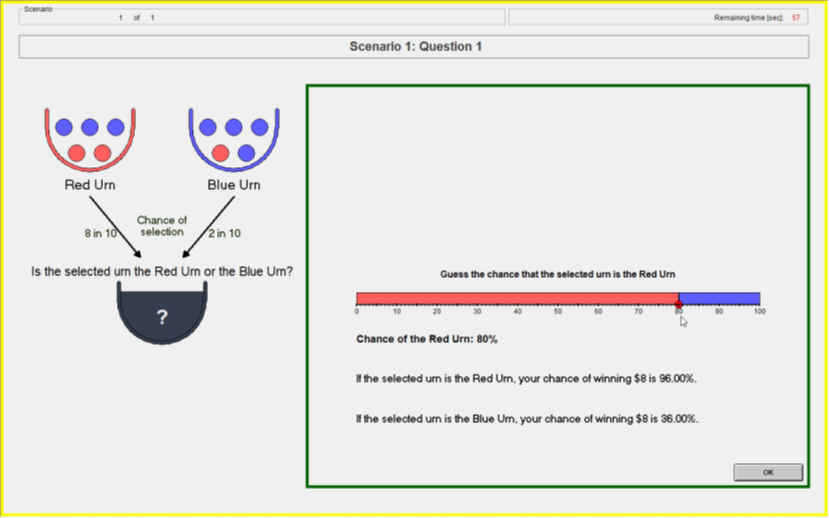
Task
Each belief scenario consists of three seperate elicitations.

- Guess 1: Prior
- Guess 2: Posterior
- Guess 3: Posterior


Initial Design
- 5 treatments
- Treatment variation: Information on incentives
- Holding constant across treatments
- Incentives
- Experimental procedures
- All scenarios and random draws matched
- 60 participants per treatment (3x20)
- Written instructions read out loud, slide summary
- 10 scenarios with random draws (30 elicitations total)
- Payment
- $8 show up
- $8 prize with one guess paid from two scenarios
- One participant per session paid for end-of-experiment elicitations
Baseline: Information Treatment
| Property | Information |
|---|---|
| Dominant Strategy | |
| Payoff Description | |
| Payoff Slider | |
| Feedback |
✅
✅
✅
✅
✅
✅
✅
✅
Dominant Strategy
Instructions:
The payment rule is designed so that you can secure the largest chance of winning the prize by reporting your most-accurate guess.
Slide summarizing instructions:
(literally the last thing they see
before they begin making decisions)
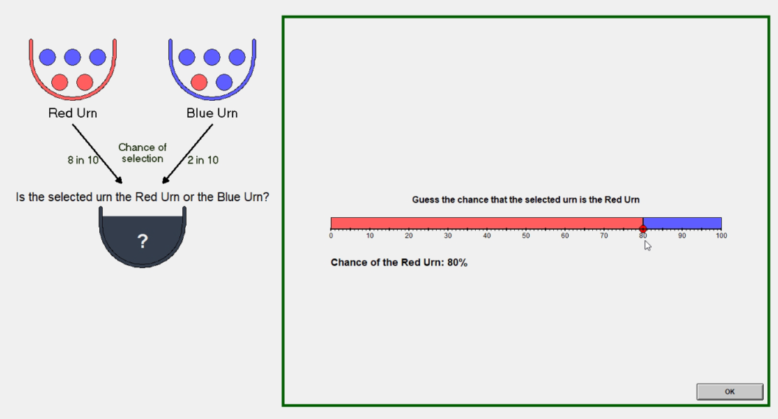
Payoff Description
- Randomly draw two uniform numbers between 0-100
- If the selected urn is the Red urn: You will win the $8 prize if Your Guess is greater than or equal to either of the two Computer Numbers.
- If the selected urn is the Blue urn: You will win the $8 prize if Your Guess is less than either of the two Computer Numbers.
- Yields the BSR lottery probabilities (Wilson & Vespa 2018)
\text{Prob}\left\{q\leq \max(U_1,U_2)\right\}=1-q^2
\text{Prob}\left\{q\geq \min(U_1,U_2)\right\}=1-(1-q)^2
Payoff Slider
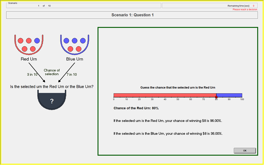
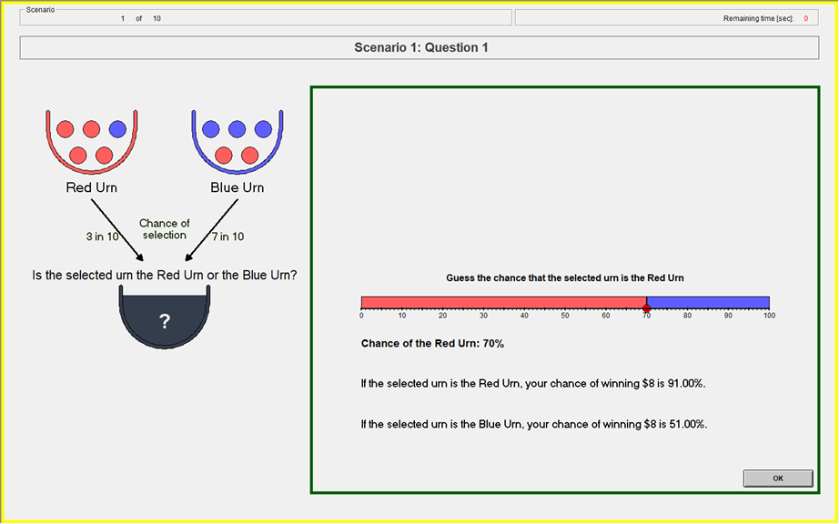
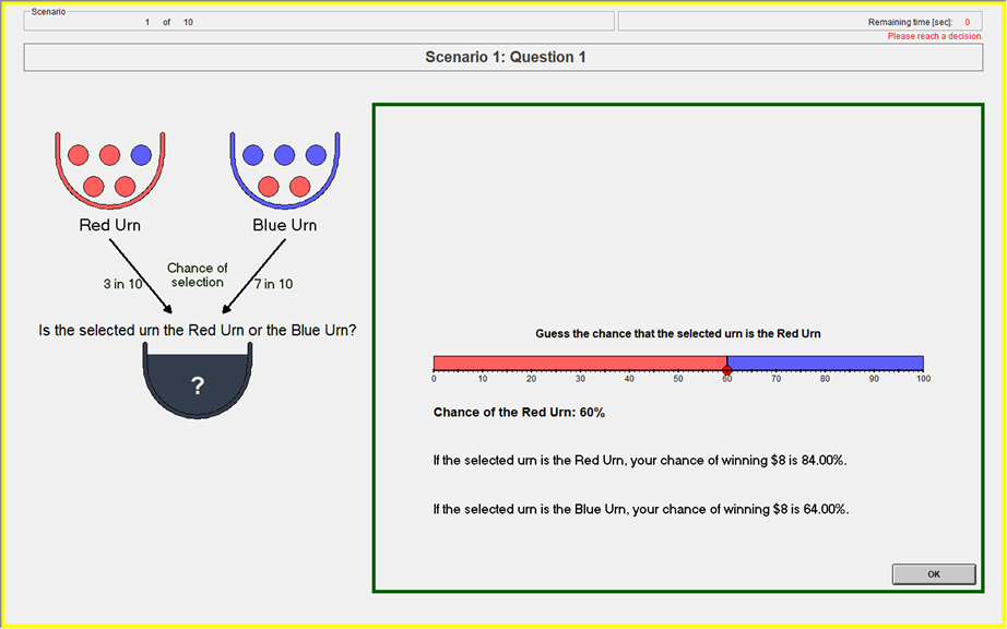
Feedback
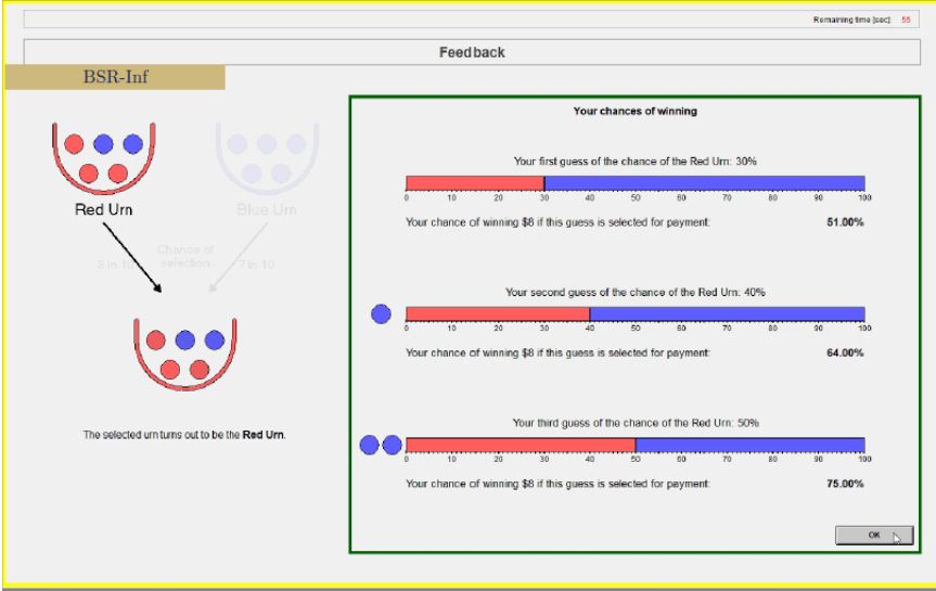
At the end of each round:
- Realized urn
- Earned probability on each elicitation
Results
-
Prior (Guess 1)
-
Posteriors (Guesses 2&3)
Guess 1: Prior Elicitation
Should report induced prior if incentivized to tell truth
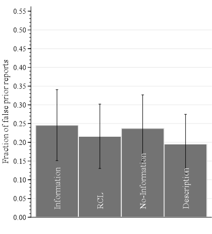
Only 15 percent of participants consistently report given prior
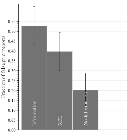
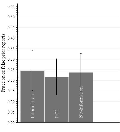
Information: False priors report
What Drives False Reports?
-
Confusion (inability/unwillingness to report given prior)
-
Incentives:
-
Failure to reduce compound lottery (RCL)
-
Payoff structure
-
BSR Payoffs
- Reporting a belief toward center
- large increase in chance of winning on unlikely event
- smaller decrease in chance of winning on likely event
84% chance
83% chance
- Cheap false reports:
- 10% pt deviation from truth reduces chance of winning by 1% pt
| Stated Belief on Red | Chance to Win if Red | Chance to Win if Blue |
|---|---|---|
| 1 | 100% | 0% |
| 0.9 | 99% | 19% |
| 0.8 | 96% | 36% |
| 0.7 | 91% | 51% |
| 0.6 | 84% | 64% |
| 0.5 | 75% | 75% |
What Drives False Reports?
-
Confusion (inability/unwillingness to report given prior)
-
Incentives:
-
Failure to reduce compound lottery (RCL)
-
Payoff structure (asymmetric and flat incentives)
-
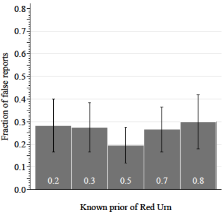
Evidence that Incentives drive False Reports
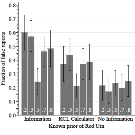
- False reports more likely on non-centered than centered priors
- Deviations more likely toward center than near extreme (reports pull-to-center)
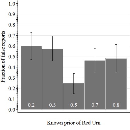


Elicited Priors at 0.3
Near-extreme
Center
Distant-extreme
False-report movements
\pi_0
\tfrac{1}{2}
0
1
47\% \text{ for } \pi_0\neq\tfrac{1}{2}
17\%
28\%
7\%
Proportion of non-centered reports in each bin:
Evidence of incentives distorting reports
- False reports more likely on non-centered than centered priors
- Pull-to-center: Deviations more likely toward center than near extreme
- Survey responses discuss a hedging motive
- Confusion
-
Incentives
-
Failure to reduce compound lottery
-
flatness
-
asymmetry
-
-
Vary information on incentives:
-
RCL-calculator : Aid reduction of compound lottery
-
No-Information: Eliminate quantitative information on incentives
-
Cause of false BSR reports?
✅
✅
✅
✅
❌
✅
✅
✅
✅
❌
Treatments:
- RCL adds information on the incentives
- No Information subtracts information
| Property | Information | RCL | No-Information |
|---|---|---|---|
| Dominant Strategy | | ||
| Payoff Description | | ||
| Payoff Slider | | ||
| Feedback | | ||
| RCL calculator | |
✅
❌
❌
❌
❌
✅
✅
✅
✅
✅

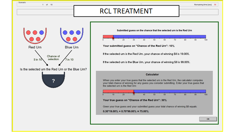
Information treatment
RCL Treatment
No Information treatment
What drives BSR false reports?
| Treatment | Source |
|---|---|
| Information | confusion, BSR incentives, failed RCL |
| RCL | confusion, BSR incentives |
| No Information | confusion |
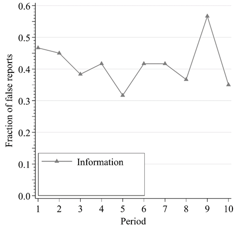
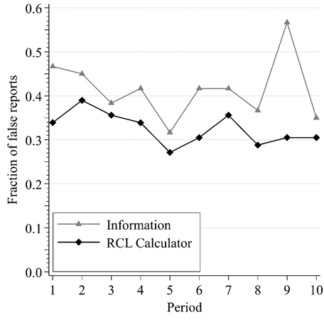
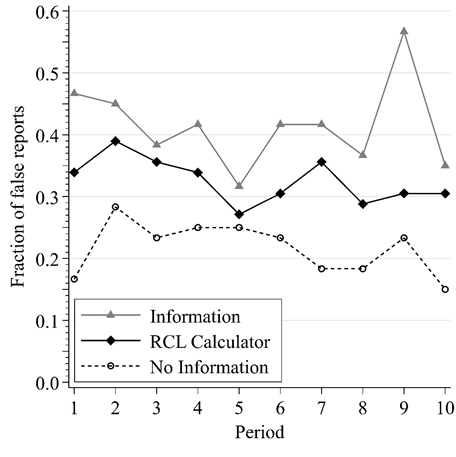
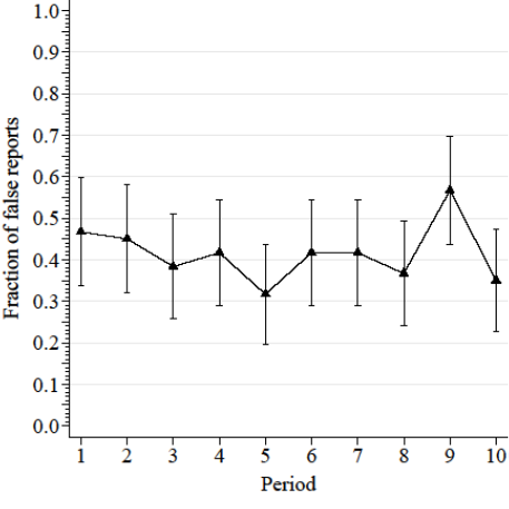
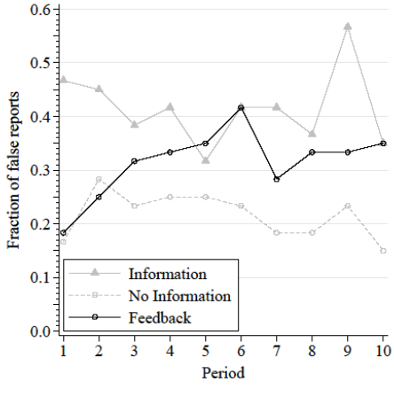
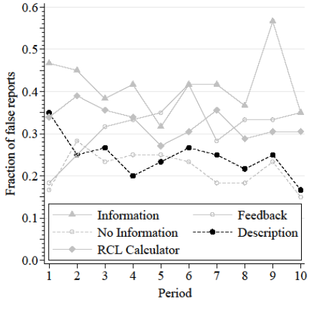
False Reports by Round
\Bigr\}
Truthful reporting greatest w/o incentive information
False reports by Prior
Near-extreme
Center
Distant-extreme
\pi_0
\tfrac{1}{2}
0
1
Proportion of non-centered reports in each bin:
Inf:
17\%
28\%
7\%
RCL:
16\%
17\%^\star
7\%
NoInf:
11\%
6\%^\star
4\%
Distribution of false reports
By prior location:
Confusion
BSR Incentives
Compounding
False reports
\pi_0\neq\tfrac{1}{2}
Centered Prior
\pi_0=\tfrac{1}{2}
BSR Incentives
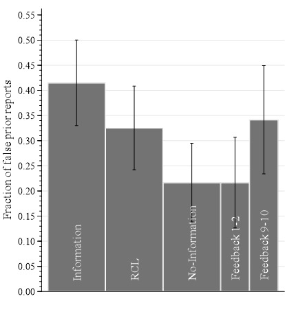
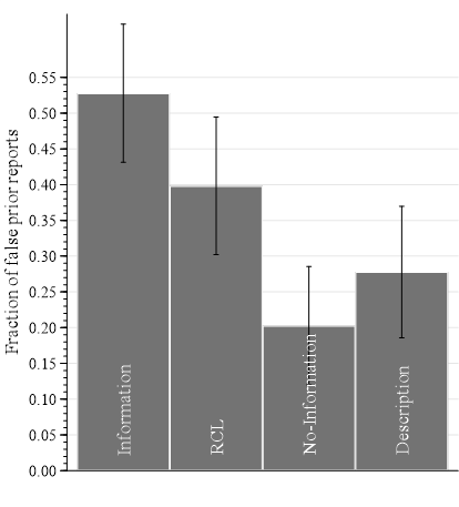
- Information on BSR incentives increases false reports (by 150%) (between-subject)
- Test effect of information within subject
- Feedback Treatment
- No-Info + scenario feedback with gradual information on incentives
- Feedback Treatment
| Property | Inf | RCL | No-Inf | Feedback |
|---|---|---|---|---|
| Dominant Strategy | ✅ | ✅ | ✅ | ✅ |
| Payoff Description | ✅ | ✅ | ❌ | ❌ |
| Payoff Slider | ✅ | ✅ | ❌ | ❌ |
| Feedback | ✅ | ✅ | ❌ | ✅ |
| RCL calculator | ❌ | ✅ | ❌ | ❌ |
Feedback Treatment
Feedback screen

False prior reports
\left(q\neq\pi_0\right)
- Starts out at No Information level
- Ends up at Information level
- Information on incentives distorts truthful reporting within subject
False Reports of Prior
Summary so far...
-
Information on incentives increases false reports
-
Between subject: Information vs. No-Information
-
Within subject: Feedback
-
-
What is ‘enough’ information to maintain truth telling?
-
Description Treatment
-
| Property | Inf | RCL | No-Inf | Feedback | Description |
|---|---|---|---|---|---|
| Dominant Strategy | ✅ | ✅ | ✅ | ✅ | ✅ |
| Payoff Description | ✅ | ✅ | ❌ | ❌ | ✅ |
| Payoff Slider | ✅ | ✅ | ❌ | ❌ | ❌ |
| Feedback | ✅ | ✅ | ❌ | ✅ | ❌ |
| RCL calculator | ❌ | ✅ | ❌ | ❌ | ❌ |
Description Treatment
Description Treatment
By round
By prior
False Reports
\pi_0=\tfrac{1}{2}
\pi_0\neq\tfrac{1}{2}
Summary
- Evidence for systematic distortions over objective priors
- When subjects are informed on the incentives they make systematic deviations
- That deviations are purposeful distortions is clearest
- But the environment is perhaps more artificial
- The same patterns are observed over Bayesian Posteriors
- Data here is harder to pinpoint as we don't know the 'true' posterior beliefs
- But distributions of response shift in same systematic way
- Two questions raised:
- Would this also hold for subjective beliefs?
- Does any of this matter for inference?
BSR Usage in Literature
- Most papers are eliciting probabilistic beliefs
- Most papers give two or more quantitative examples of the incentives
- Usage for beliefs is both as a LHS and RHS variable
EU assumption is used at observation level!
- EU in standard economic theory is typically used at an aggregate (i.e. average) level
- Predict a comparative static for a population
- But in the elicitation EU is used at the observation level:
- Use the IC under EU to interpret a choice over incentives as a measured belief
- 'Small' mistakes in the EU assumption can lead to a measurement error for any inference
- Regressions using mismeasured data can cause biased inference
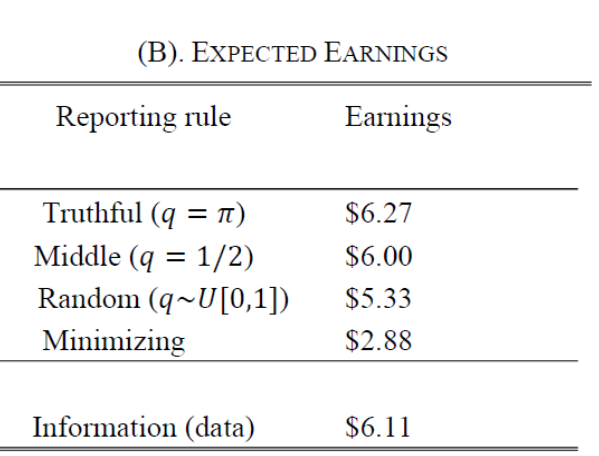
Inferential Effects
To understand the effects on inference we use a simple model of the center-bias distortions
Observed belief is:
{\color{red}q}=
\begin{cases}
{\color{blue}q^\star} \text{ (true belief)} & \text{with prob. }\alpha\\
c \text{ (center point)} & \text{with prob. }1-\alpha
\end{cases}
\text{RHS: }y_i=\mu_y+\delta_{y}\cdot X_i + \beta_{q} \cdot {\color{red}q_i} +\epsilon_y
\text{LHS: }{\color{red}q_i} = \mu_{q}+\delta_{q} \cdot X_i+\epsilon_q
\text{RHS: }y_i=\mu_y+\delta_{y}\cdot X_i + \beta_{q} \cdot {\color{blue}q^\star_i} +\epsilon_y
\text{LHS: }{\color{blue}q^\star_i} = \mu_{q}+\delta_{q} \cdot X_i+\epsilon_q
Regression model where X is a binary treatment indicator:
What happens when distorted beliefs are used?
Inferential Effects
Observed belief is:
{\color{red}q}=
\begin{cases}
{\color{blue}q^\star} \text{ (true belief)} & \text{with prob. }\alpha\\
c \text{ (center point)} & \text{with prob. }1-\alpha
\end{cases}
\text{LHS: }{\color{red}q_i} = \mu_{q}+\delta_{q} \cdot X_i+\epsilon_q
Left-hand-side effect is clear:
- Mismeasurement of q leads to an attenuation of the estimated treatment effect
\left|\mathbb{E}\left(\hat{\delta}_q\right)\right|< \left|\delta_q\right|
Inferential Effects
Observed belief is:
{\color{red}q}=
\begin{cases}
{\color{blue}q^\star} \text{ (true belief)} & \text{with prob. }\alpha\\
c \text{ (center point)} & \text{with prob. }1-\alpha
\end{cases}
\text{RHS: }y_i=\mu_y+\delta_{y}\cdot X_i + \beta_{q} \cdot {\color{red}q_i} +\epsilon_y
Right-hand-side treatment effect will depend on unknowns:
\text{Asym. Bias}\left(\hat{\delta}_y(\alpha)\right)=\beta_ {q}\cdot \delta_q \frac{\alpha+\alpha\Delta^2}{1+\alpha \cdot \Delta^2}
\text{Asym. Bias}\left(\hat{\beta}_q(\alpha)\right)=-\frac{\alpha \Delta^2}{1+\alpha \cdot \Delta^2}\beta_q
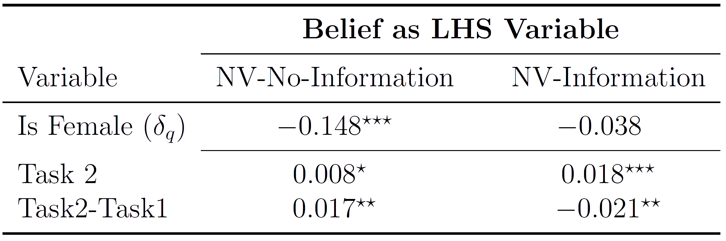
Niederle & Vesterlund (2006)
We return to the Niederle & Vesterlund study:
- Perform sums for a piece rate
- Perform sums in tournament
- Choose the preferred incentive
- Elicit subjective belief
- (here using BSR)
Run this study twice:
- NV-Information: Quantitative information
- NV-No-Information : No precise information
\text{Enter}_i=\mu_y+\delta_{y}\cdot \text{IsFemale}_i + \beta_{q} \cdot {\color{red}\text{Belief}_i} +\epsilon_y
{\color{red}\text{Belief}_i} = \mu_{q}+\delta_{q} \cdot \text{IsFemale}_i+\epsilon_q
LHS: Confidence difference between men and women:
RHS: Competition difference for men and women after controlling for confidence:
NV Inference equations
Information predicted to attenuate gender confidence difference
Information predicted to make the gender-gap in tournament-entry larger (after controlling for confidence
Elicited Beliefs


NV-No-Information
NV-Information
Elicited Beliefs
NV-No-Information
NV-Information
NV-Regressions LHS
Original finding is that:
- Women are less confident over their performance than men
- Prediction from model for NV-Information is that gender gap will move towards zero.
\delta_q<0
NV-Regressions RHS
- Original finding is that:
- Beliefs explain a significant proportion of the gender gap
- Prediction from model for NV-Information is that gender gap in competition is more negative:
- (gender gap in confidence)
- (Belief effect on entry)
\delta_q<0
\beta_q>0
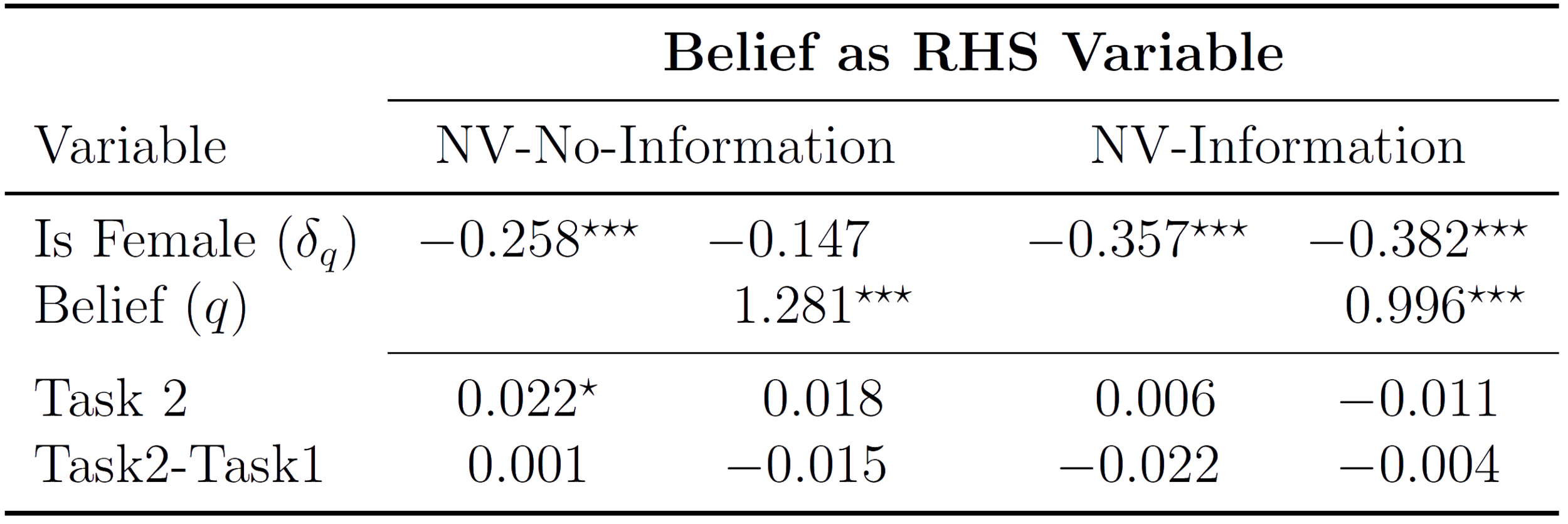
\left(\text{bias-sign}=\text{sign}\left(\beta_q\cdot\delta_q\right)\right)
NV Replication Results
- NV-Information distorts beliefs to center, relative to NV-No-Information
- This difference in the beliefs affects final inference:
- As a LHS variable it attenuates the treatment effect (here a gender gap over beliefs)
- As a RHS variable it widens the measured gender gap over competition after controlling for beliefs
- So, simply by providing the participants with information on the elicitation incentives, that we can qualitatively distort the subsequent inference
Going Forward...
- The BSR does not work as an incentive-compatible elicitation
- The less you tell the participants about the incentives, the worse the data
- This is true for:
- Objective priors
- Updated posteriors
- Subjective beliefs
- New elicitations are required. But how should we go about assessing them?
Propose two weak tests for behavioral incentive compatibility
- The mechanism should not yield worse data when participants are given precise information on the incentives on offer
- If presented with the pure incentives available in the mechanism, the majority of participants should be choosing the theorized maximizer
Weak Condition 1:
BIC Diagnostic 1:
- Information vs No Information comparison
Our paper demonstrates this methodology across:
- Elicitation of an objective prior
- Elicitation of an objective posterior
- Elicitation of a subjective belief
Have similar data showing this comparison for:
- Quadratic scoring rule
- Binarized-BDM
Weak Condition 2:
BIC Diagnostic 2:
- Extract the pure incentives from the elicitation and ask the participants to choose. A majority should be choosing the theorized maximizer
| Lottery pair | Red lottery ticket | Blue lottery ticket |
|---|---|---|
| A (0%) | 100% | 0% |
| B (10%) | 99% | 19% |
| C (20%) | 96% | 36% |
| D (30%) | 91% | 51% |
| E (40%) | 84% | 64% |
| F (50%) | 75% | 75% |
| G (60%) | 64% | 84% |
| H (70%) | 51% | 91% |
| I (80%) | 36% | 96% |
| J (90%) | 19% | 99% |
| K (100%) | 0% | 100% |
Fix the probability of Red and ask for a choice from:
Weak Condition 2:
We asked 120 subjects to choose their preferred lottery pair when the probability of Red was set to either 20% or 30%. Interpret choice via the EU assumption:
\Pr\left\{\text{Red}\right\}=0.2
\Pr\left\{\text{Red}\right\}=0.3


Weak Condition 2:
Same thing, but for QSR incentives:
\Pr\left\{\text{Red}\right\}=0.2
\Pr\left\{\text{Red}\right\}=0.3


Weak Condition 2:
Same thing, but for binarized-BDM (Karni)
\Pr\left\{\text{Red}\right\}=0.2
\Pr\left\{\text{Red}\right\}=0.3


Weak Condition 2:
First Price Auction, two bidders, uniform values:
\[v^\star=0.3\]
| Lottery pair | Prize | Probability |
|---|---|---|
| A (v=0.0) | $12 | 0% |
| B (v=0.1) | $10 | 10% |
| C (v=0.2) | $8 | 20% |
| D (v=0.3) | $6 | 30% |
| E (v=0.4) | $4 | 40% |
| F (v=0.5) | $2 | 50% |
| G (v=0.6) | $0 | 60% |
| H (v=0.7) | -$2 | 70% |
| I (v=0.8) | -$4 | 80% |
| J (v=0.9) | -$6 | 90% |
| K (v=1.0) | -$8 | 100% |
Weak Condition 2:
First Price Auction, two bidders, uniform values:
\[v^\star=0.7\]
| Lottery pair | Prize | Probability |
|---|---|---|
| A (v=0.0) | $28 | 0% |
| B (v=0.1) | $26 | 10% |
| C (v=0.2) | $24 | 20% |
| D (v=0.3) | $22 | 30% |
| E (v=0.4) | $20 | 40% |
| F (v=0.5) | $18 | 50% |
| G (v=0.6) | $16 | 60% |
| H (v=0.7) | $14 | 70% |
| I (v=0.8) | $12 | 80% |
| J (v=0.9) | $10 | 90% |
| K (v=1.0) | $8 | 100% |
Weak Condition 2:


\[v^\star =0.3\]
\[v^\star =0.7\]
First Price Auction:
Weak Condition 2:
Uniform Preferences
Correlated Preferences
Deferred Acceptance (Proposing over $6/$4/$2)
Assume all other players truthfully reveal
- Two other proposers
- Three prize amounts
Weak Condition 2:
Uniform Preferences
Deferred Acceptance (Proposing over $6/$4/$2)
| Lottery pair | $8 | $6 | $2 | $0 |
|---|---|---|---|---|
| A (6>8>2) | 26% | 64% | 10% | 0% |
| B (6>8>2) | 26% | 64% | 0% | 10% |
| C (6>2>8) | 10% | 64% | 26% | 0% |
| D (6>2) | 0% | 64% | 26% | 10% |
| E (8>6>2) | 64% | 26% | 10% | 0% |
| F (8>6) | 64% | 26% | 0% | 10% |
| G (8>2>6) | 64% | 10% | 26% | 0% |
| H (8>2) | 64% | 0% | 26% | 10% |
| I (2>6>8) | 10% | 26% | 64% | 0% |
| J (2>6) | 0% | 26% | 64% | 10% |
| K (2>8>6) | 26% | 10% | 64% | 0% |
| L (2>8) | 26% | 0% | 64% | 10% |
Weak Condition 2:
Correlated Preferences
Deferred Acceptance (Proposing over $6/$4/$2)
| Lottery pair | $8 | $6 | $2 | $0 |
|---|---|---|---|---|
| A (6>8>2) | 9% | 64% | 29% | 0% |
| B (6>8) | 9% | 64% | 0% | 29% |
| C (6>2>8) | 1% | 64% | 36% | 0% |
| D (6>2) | 0% | 64% | 36% | 1% |
| E (8>6>2) | 41% | 33% | 26% | 0% |
| F (8>6) | 41% | 33% | 0% | 26% |
| G (8>2>6) | 41% | 7% | 52% | % |
| H (8>2) | 47% | 0% | 52% | 7% |
| I (2>6>8) | 1% | 8% | 91% | 0% |
| J (2>6) | 0% | 8% | 91% | 1% |
| K (2>8>6) | 2% | 7% | 91% | 0% |
| L (2>8) | 2% | 0% | 91% | 7% |
Weak Condition 2:
Uniform Preferences
Correlated Preferences
Deferred Acceptance (Proposing over $6/$4/$2)


Conclusions
- On the Binarized Scoring Rule
- Substantial false-report rate for objective prior
- Systematic deviations driven by information on the incentives
- Between (Information vs No Information)
- Within (gradual Feedback)
-
Distortions generated can qualitatively affect inference
-
Replication of Niederle & Vesterlund fails when incentive information present
-
Conclusion
- Overly content to appeal to theoretical incentive compatibility, when what is actually required are notions of behavioral compatibility
- For belief elicitation, qualitative notions are effective:
- Both No Information and Description work well
- But need to ask ourselves if it truly the incentives, instead of framing/call to authority
- Might want to ask if it even makes sense to collect arbitrarily precise beliefs.
- Methodology offers simply diagnostic checks for behavioral incentive compatibility
- Simple demonstrations for check on First Price auctions and Matching mechanisms
B-IC (Exter)
By Alistair Wilson


