Binary Classifier Two-Sample Test (C2STs) with Logistic Regression
CPSC 532S - Danica Sutherland
James, Amin, James
Spring 2022
Two Sample Tests - Motivation
P = Q?
Two Sample Tests - Motivation
Two Sample Tests - The Basics
H_0 (\text{Null Hypothesis}) \rightarrow P=Q
S_p := \{x_1, ..., x_n\} \sim_{i.i.d} P^n(X)
S_q := \{y_1, ..., _yn\} \sim_{i.i.d} Q^n(Y)
H_1 (\text{Null Hypothesis}) \rightarrow P\neq Q
Two Sample Tests - The Basics cont.
Steps to the standard two-sample test:
1) determine a significance level as input to the test
2) manually compute the test statistic
3) compute p-value
4) reject the null hypothesis if our calculated p value is less than alpha, and fail to do so otherwise.
\alpha \in [0,1]
\hat{t} = \frac{|\bar{\mu_{S_p}} – \bar{\mu_{S_q}}|} {\sqrt{\frac{\bar{\sigma{S_p}}}{n_{S_p}} + \frac{\bar{\sigma{S_p}}}{n_{S_p}}}}
\hat{p} = Pr(T \geq \hat{t} | H_0)
C2STs - Classifier Two Sample Tests
D = {(x_i, 0)}_{i=1}^n \bigcup {(y_i, 1)}_{i=1}^n =: {(z_i, l_i)}_{i=1}^{2n}
Shuffle D at random and split it into training and test subsets
D = D_{tr} \cup D_{te}, D_{tr} \cap D_{te} = \text{\O}
n_{te} = |D_{te}|
"Revisiting Classifier Two-Sample Tests "[Lopez-Paz and Oquab, 2016]
C2STs - Classifier Two Sample Tests cont.
Train a binary classifier
f: X \rightarrow{} [0,1] \text{ on } D_{tr}
\hat{t} = \frac{1}{n_{te}} \sum_{(z_i, l_i) \in D_{te}} \mathbb{I} [\mathbb{I} [f(z_i) > \frac{1}{2}] = l_i]
\frac{\text{number of examples correctly labeled}}{\text{total number of examples}} = 1 - L_{D_te}^{0-1} (\mathbb{I}[f(z_i) > \frac{1}{2}])
C2STs - Classifier Two Sample Tests cont.
From here we develop the p value as is traditionally done in normal two sample tests
\hat{p} = Pr(T \geq \hat{t} | H_0)
\mathbb{I} [\mathbb{I} [f(z_i) > \frac{1}{2}] = l_i]
H_0 \rightarrow{} N(\frac{1}{2}, \frac{1}{4 n_{te}})
H_1 \rightarrow{} N(\bar{p}, \frac{\bar{p}(1-\bar{p})}{n_{te}})
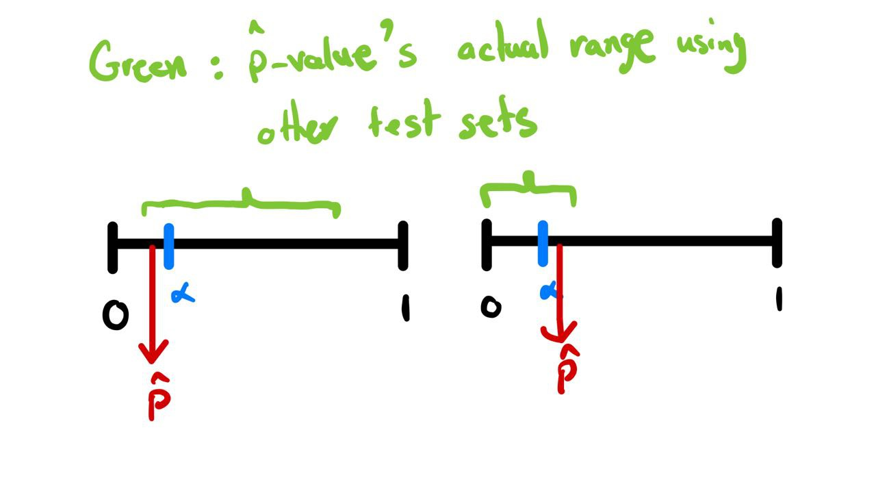
Theoretical Motivation
Finding bounds for p-value
- Imagine we have trained a classifier on our data.
- We then compute the (pseudo) t-statistic using a test set .
- Then we calculate the p-value using the following function:
- But, how confident are we that our p-value will be almost the same, if we change the test set?
- Possible scenarios in the next slide.
D_{te}
\Gamma(t) = Pr(T \ge t | H_0)
Finding bounds for p-value
Finding Bounds: Linear Classifiers
- Let's start with a simple case:
- Take the space of linear classifiers:
- Use 0-1 loss:
- Let's derive the (pseudo) t-statistic of this classifier:
- Note that:
- Idea: if we find some bounds for , we can use them to find bounds for our reported p-value.
\mathcal{H} = \{\langle w, x \rangle\}
l(h, (x, y)) = \mathbb{I}(sign(h(x)) = y)
\hat{t} = \frac{1}{n_{te}}\sum_{(x, y) \sim D_{te}}\mathbb{I}(sign(h(x)) \ne y)
L^{0-1}_{D_{te}}(h) = 1 - \hat{t}
L^{0-1}_{D_{te}}(h)
Finding Bounds for Linear Classifiers: Test Loss
- Let's start with the Uniform Convergence of Linear Classifiers trained with 0-1 loss:
-
We have the assumptions that:
-
We know that
-
Thus: [https://cse.buffalo.edu/~hungngo/classes/2011/Fall-694/lectures/rademacher.pdf]
-
Using this, we can derive the uniform convergence bounds:
\mathcal{H} = \{\langle w, x \rangle\} \qquad \mathcal{G} = {\ell^{0-1} \circ \mathcal{H}}
VCdim(\mathcal{H}) = d \Longrightarrow \mathcal{R}_n(\mathcal{H}) \le \sqrt{\frac{2\, d \, log(n)}{n}}
\mathcal{R}_n(\mathcal{G}) \le \frac{1}{2} \sqrt{\frac{2\, d \, log(n)}{n}} + \frac{1}{2\sqrt{n}}
\Longrightarrow \sup_{h\in\mathcal{H}} | L^{0-1}_S(g)) - L^{0-1}_D(g))| \le \sqrt{\frac{2\, d \, log(n)}{n}} + \frac{1}{\sqrt{n}} + \sqrt{\frac{1}{2n} \log\frac{1}{\delta}} \text{ w.p. } 1-\delta
Finding Bounds for Linear Classifiers: Test Loss
- But, how do we derive bounds for test loss?
-
Remember that:
-
Combining this with the uniform convergence property, we get:
- Remember that
- We get:
- Note that is a monotonically decreasing function, Thus:
L^{0-1}_S(g) - \varepsilon_1(n, \delta_1) - \varepsilon_2(n_{te}, \delta_2) \le L^{0-1}_{D^{te}}(g) \le L^{0-1}_S(g) + \varepsilon_1(n, \delta_1) + \varepsilon_2(n_{te}, \delta_2)
|L_{V}(h) - L_{D}(h)| \le \sqrt{\frac{1}{2|V|}\log\frac{2}{\delta}} \text{ w.p. } 1-\delta
L^{0-1}_{D_{te}}(g) = 1-\hat{t}
t_{tr} - \varepsilon_1(n, \delta_1) - \varepsilon_2(n_{te}, \delta_2) \le \hat{t} \le t_{tr} + \varepsilon_1(n, \delta_1) + \varepsilon_2(n_{te}, \delta_2)
\Gamma(t) = 1 - CDF_{N(0, 1)}(t)
\Gamma(t_{tr} + \varepsilon(n^*, \delta^*)) \le \hat{p} \le \Gamma(t_{tr} - \varepsilon(n^*, \delta^*)) \text{ w.p. } 1 - \delta^*
Finding Bounds for Logistic Regression
- But, we can't really train classifiers on 0-1 loss.
- How about logistic loss? (Logistic Regression)
- Well, the (pseudo) t-statistic and the p-value computations are based on 0-1 loss...
- We would have to design a new test for other (pseudo) t-statistics.
- Idea: Use logistic loss as a surrogate loss for 0-1 Loss.
- The good: bounds for logistic regression!!!
- The ugly: One-sided bounds for logistic regression :(
- Because the surrogate loss bounds 0-1 loss only on one side
Finding Bounds for Logistic Regression
-
We showed that:
-
Note that:
-
Thus:
-
Which gives us:
- We have derived a one-sided bound on the p-value of our test, when our classifier is a linear classifier trained with logistic loss (logistic regression).
L^{0-1}_s(g) \le L_S^{log}(g) \Longrightarrow 1- L^{0-1}_s(g) \ge 1-L_S^{log}(g) \Longrightarrow t_{tr} \ge t_{tr}^{log}
t_{tr} - \varepsilon_1(n, \delta_1) - \varepsilon_2(n_{te}, \delta_2) \le \hat{t} \le t_{tr} + \varepsilon_1(n, \delta_1) + \varepsilon_2(n_{te}, \delta_2)
t^{log}_{tr} - \varepsilon_1(n, \delta_1) - \varepsilon_2(n_{te}, \delta_2) \le \hat{t}
\hat{p} \le \Gamma(t^{log}_{tr} - \varepsilon(n^*, \delta^*)) \text{ w.p. } 1 - \delta^*
Experiments
Experiment Detail
-
Implemented Logistic Regression in Pytorch
-
Tested on synthetic data sampled from 1D distributions
-
Trained for 200 epochs on 400 generated examples
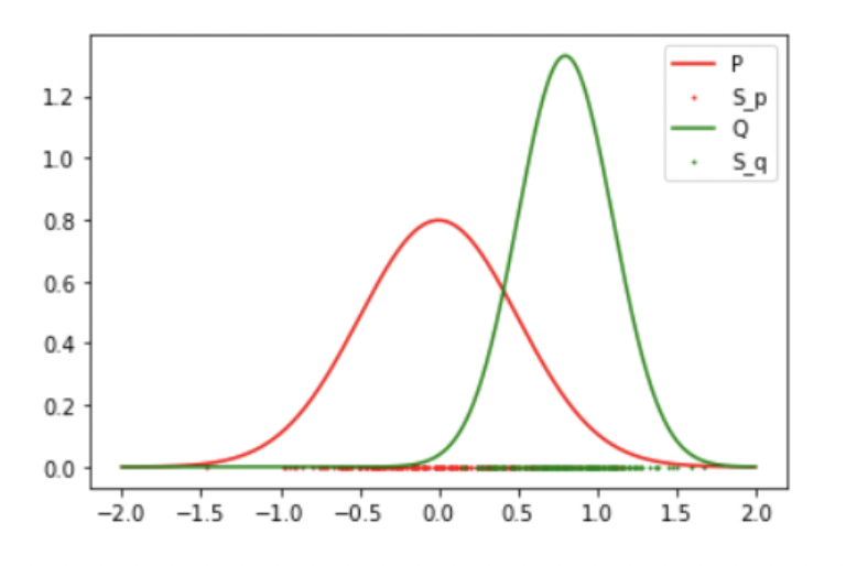
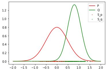
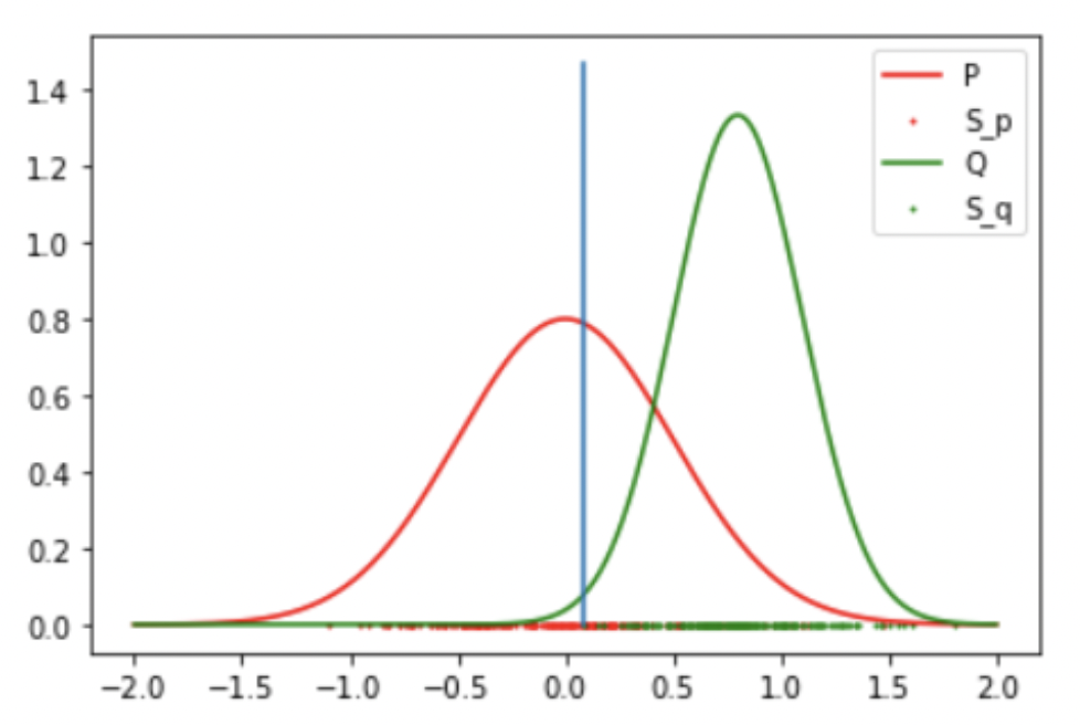
Results: 2 Gaussian (Success)
-
Result: Reject the Null Hypothesis, P != Q
-
Mean: 0 std: 0.5
-
Mean: 0.8 std: 0.3
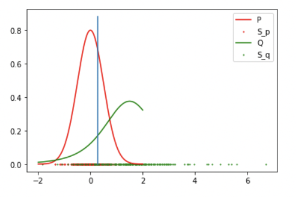
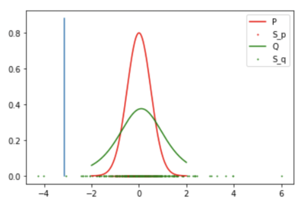
Result 3: Gaussian and Student T (Success)
-
Result: Reject the Null Hypothesis, P = Q
-
Mean: 0 std: 0.5
-
Student T: DoF: 4 mean: 1.5
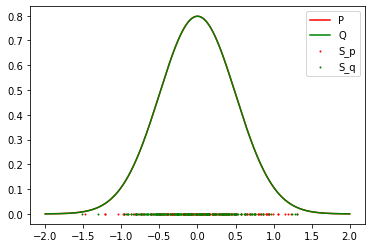
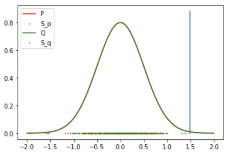
Results: 1 Gaussian (Success)
-
Result: Accept the Null Hypothesis, P = Q
-
Mean: 0 std: 0.5
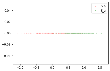
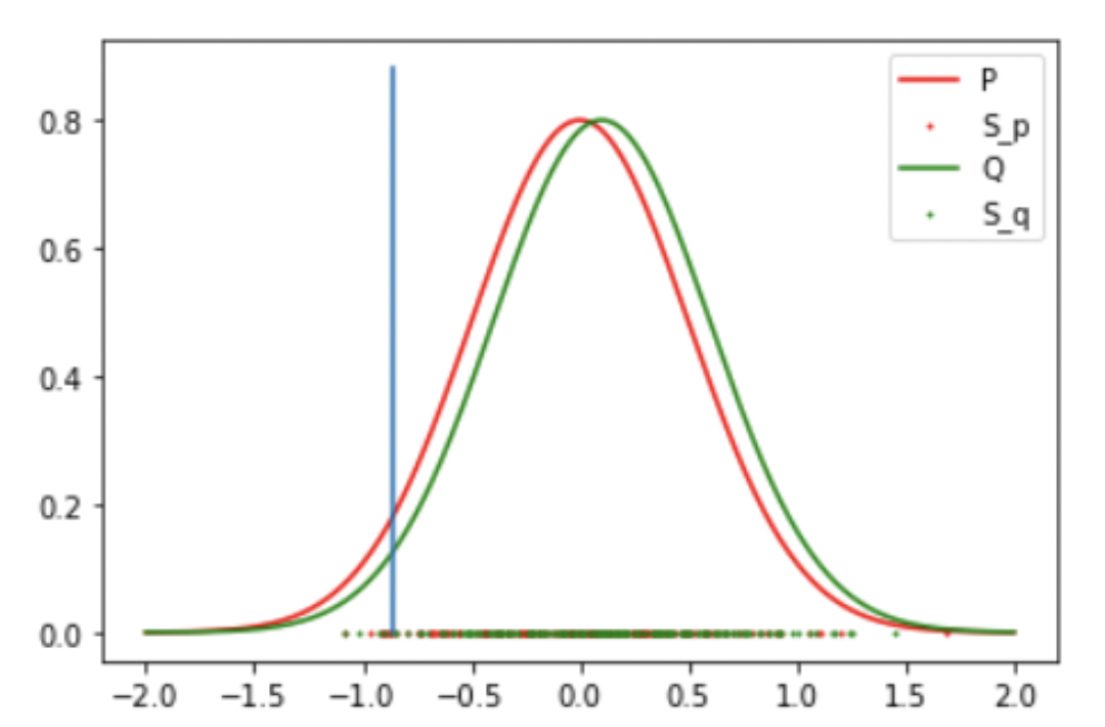
Result 3: 2 Gaussian (False Negative)
-
Result: Accept the Null Hypothesis, P = Q
-
Gaussian: Mean: 0 std: 0.5
-
Student T: DoF: 4 mean: 0.1
Result 3: Gaussian and Student T (False Negative)
Result: Accept the Null Hypothesis, P = Q
-
Gaussian: Mean: 0 std: 0.5
-
Student T: DoF: 4 mean: 0.1
Thanks!
Copy of Binary Classification Two-Sample Test (C2STs) with Logistic RegressionCPSC 532S - Danica Sutherland
By Amin Mohamadi


