A fast, well founded approximation to the empirical NTK, and its application in “look-ahead” deep active learning
Mohamad Amin Mohamadi
The University of British Columbia
March 2023

Outline of the talk
-
Empirical Neural Tangent Kernels
-
Approximating eNTKs
- Pseudo-NTKs: One logit might be enough!
- Bounds on approximation error
- Empirical evidence
- Surprising behaviours
-
Applications: "Look-Ahead" Deep Active Learning
- Active Learning
- Using eNTKs to approximate re-training NNs
- Empirical evaluations
The Neural Tangent Kernel
-
An important object in characterizing the training of suitably-initialized infinitely wide neural networks (NN)
-
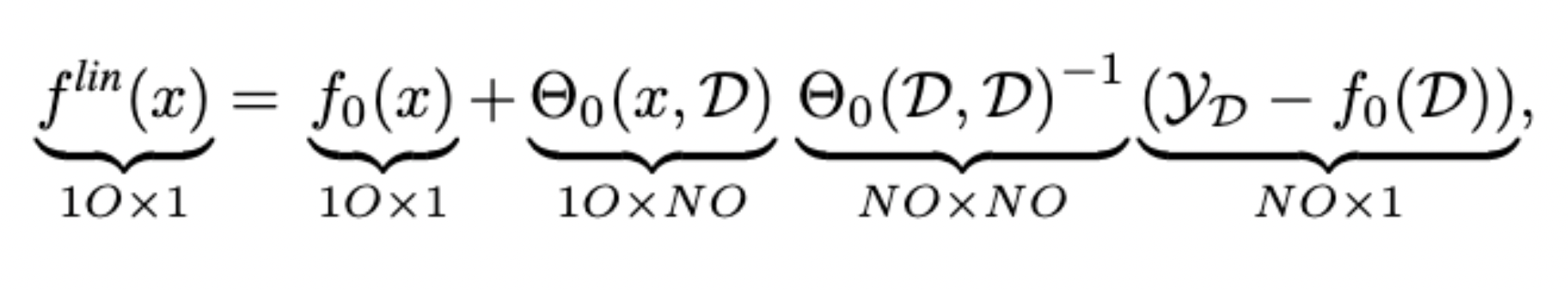
Describes the exact training dynamics of first-order Taylor expansion of any finite-width neural network:
- Is defined as
\Theta_\theta(x_1, x_2) = J_\theta f_\theta(x_1) {J_\theta f_\theta(x_2)}^\top
f_t(x) = f_0(x) + \Theta_f(x, \mathcal X) {\Theta_\theta}^{-1} (I - e^{-t\Theta_\theta})(\mathcal Y - f_0(\mathcal X))
1: Jacot, A., Gabriel, F., and Hongler, C. Neural tangent kernel: Convergence and generalization in neural networks.
2: Lee, J., Xiao, L., Schoenholz, S., Bahri, Y., Novak, R., SohlDickstein, J., and Pennington, J. Wide neural networks of any depth evolve as linear models under gradient descent.
[1]
[2]
The (Empirical) NTK
-
Is, however, notoriously expensive to compute :(
-
Both in terms of computational complexity, and space complexity!
- Computing the Full empirical NTK of ResNet18 on CIFAR-10 requires over 1.8 terabytes of Memory !
-
Our contribution:
- Pseudo-NTK: An approximation to the eNTK, dropping the O term from the above equations!
\underbrace{\Theta_\theta(\mathcal X_1, \mathcal X_2)}_{N_1 O \times N_2 O} = \underbrace{J_\theta f_\theta(\mathcal X_1)}_{N_1 \times O \times P} \times \underbrace{{J_\theta f_\theta(\mathcal X_2)}^\top}_{P \times O \times N_2}
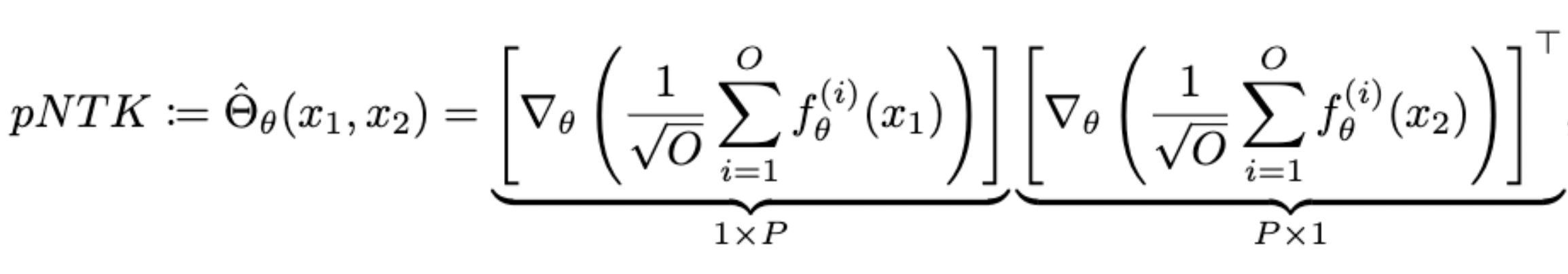
Pseudo-NTK: Definition
- For each NN, we define pNTK as follows:
- We call this sum-of-logits pNTK. We can accordingly also define single-logit pNTK.
- Computing this approximation requires \(\mathcal O(O^2)\) less time and memory complexity in comparison to the eNTK. (Yay!)
Pseudo-NTK: Motivation
- Although eNTKs in general are dense (as opposed to diagonal) matrices, in practical architectures, they become block-diagonal in expectation.
- Many recent works have thus used pNTK-like approximations in their experimental evaluations, with little to no justification.
- Question: Can we rigorously derive error bounds between pNTK and eNTK?
\mathbb E_{\theta} [ \Theta_\theta(x_1, x_2) ] = \mathbb E_\theta [\hat \Theta_\theta(x_1, x_2)] \times I_{O}
*: Under suitable parameterization at initialization, with expectation taken over the parameters of the neural network.
*
Approximation Error: Fro Norm
\Large\dfrac{{|| \Theta_\theta(x_1, x_2) - \hat\Theta_\theta(x_1, x_2) \times I_{O} ||}_F }{{||\Theta_\theta(x_1, x_2)||}_F} = \mathcal O \Big( \dfrac{1}{\sqrt{n}} \Big)
-
Theorem 1: Consider a fully-connected neural network whose parameters are initialized according to Standard Parameterization (fan_in). The following equality holds w.h.p over random initialization:
where \(n\) denotes the width of network.
-
Notes:
- This only applies to networks at initialization, but we present empirical evidence for trained weights.
- We focus on ReLU activation.
Approximation Error: Proof Idea
- Exploit the recursive structure of eNTKs in the last layer:
\Theta^{(L+1)}_{ij}(x_1, x_2) = W_i^\top \Theta^{(L)}(x_1, x_2) W_j + I(i=j) \; {f^{(L)}(x_1)}^\top {f^{(L)}(x_2)}
Pr \Big\{ \big|x^\top A x - \mathbb E[x^\top A x] \big| \ge t \Big\} \le 2 \exp \Big(-\dfrac{ct^2}{\nu^2 {||A||}_F^2 + \nu t {||A||}_F } \Big)
- Apply the Hanson-Wright Inequality:
- For any \(\nu\)-subgaussian random vector \(x\), and square matrix \(A\), there is a constant \(c\) such that:
- For simplicity, we focus on the single-logit pNTK, but the same exact proof can be applied to sum-of-logits pNTK.
Approximation Error: Fro Norm
- Define the difference matrix:
D_{ij}(x_1, x_2) = \Theta^{(L+1)}_{ij}(x_1, x_2) - {\hat \Theta^{(L+1)}_k(x_1, x_2) \times I_O}_{ij} \\[5pt]
\qquad \qquad \qquad \qquad \qquad \quad = \begin{dcases}
W_i^\top \Theta^{(L)}(x_1, x_2) W_i - W_k^\top \Theta^{(L)}(x_1, x_2) W_k & \text{if } i = j \\
W_i^\top \Theta^{(L)}(x_1, x_2) W_j & \text{if } i \ne j
\end{dcases}
- Using Hanson-Wright Inequality, derive individual high probability bounds on each entry of the difference matrix, and apply a union bound on them to bound the Frobenius Norm!
Approximation Error: Fro Norm
- For diagonal entries:
\begin{aligned}
D_{ii}(x_1, x_2) &= W_i^\top \Theta^{(L)} W_i - W_k^\top \Theta^{(L)} W_k \\
&= (W_i - W_k)^\top \Theta^{(L)} (W_i + W_k) \underbrace{- W_i^\top \Theta^{(L)} W_k + W_k^\top \Theta^{(L)} W_i}_{\; =0 \text{ as } \Theta^{(L)} \text{ is symmetric!}} \\
&= \begin{bmatrix} W_i \\ W_k \end{bmatrix}^\top \underbrace{\Bigg( \begin{bmatrix} I_n \\ -I_n \end{bmatrix} \Theta^{(L)} \begin{bmatrix} I_n & -I_n \end{bmatrix} \Bigg)}_{{\Theta^{(L)}}^*} \begin{bmatrix} W_i \\ W_k \end{bmatrix}
\end{aligned}
- For diagonal entries:
\big|D_{ii}(x_1, x_2) \big| \le \dfrac{||{\Theta^{(L)}}^*(x_1, x_2)||_F}{n} \log \dfrac 2 \delta
- Hence, with probability at least \(1-\delta\), we have that:
Approximation Error: Fro Norm
- Likewise, for off-diagonal entries:
\begin{aligned}
|D_{ij}(x_1, x_2)| &= |W_i^\top \Theta^{(L)} W_j| \le \dfrac{||{\Theta^{(L)}}(x_1, x_2)||_F}{n} \log \dfrac 2 \delta
\end{aligned}
with probability at least \(1-\delta\).
- Applying a union-bound on the off-diagonal elements yields:
with probability at least \(1-\delta\).
\begin{aligned}
\forall i \ne j; \; |D_{ij}(x_1, x_2)| \le \dfrac{||{\Theta^{(L)}}(x_1, x_2)||_F}{n} \log \dfrac{2O^2}{\delta}
\end{aligned}
Approximation Error: Fro Norm
- Applying a union bound on the entries of \(D(x_1, x_2)\) yields with probability at least \(1-\delta\):
\begin{aligned}
||D(x_1, x_2)||_F \le \dfrac{||{\Theta^{(L)}}(x_1, x_2)||_F + 4\sqrt{n}}{n} O \log \dfrac{2O^2}{\delta}
\end{aligned}
- Using the recursive definition for eNTK, we can see that for ReLU FCNs at initialization, \(||\Theta^{(L)}||_F = \mathcal O(n\sqrt{n}) \), and \(\text{Tr}(\Theta^{(L)}) = \Theta(n^2) \) w.h.p.
- Thus, with probability at least \(1-\delta\) (up to constants):
\begin{aligned}
\dfrac{||D(x_1, x_2)||_F}{||\Theta^{(L+1)}(x_1, x_2)||_F} \le \dfrac{||{\Theta^{(L)}}(x_1, x_2)||_F + 4\sqrt{n}}{\text{Tr}(\Theta^{(L)})} O \log \dfrac{2O^2}{\delta}
\end{aligned}
Approximation Error: Fro Norm
- Using the recursive definition, for \(l \in [2, L]\):
\begin{aligned}
||\Theta^{(L)}(x_1, x_2)||_F &\le \; ||V^\top \Theta^{(L-1)}(x_1, x_2) V||_F \\
& \; \; \; + || {f'^{(L-1)}(x_1)}^\top {f'^{(L-1)}(x_2)} \times I_n ||_F \\
& \le ||\Theta^{(L-1)}||_F + \sqrt{n^2 \times n}
\end{aligned}
-
Note: It's easy to see that in the fan_in mode, the dot-product of post-activations are \(\Theta(n)\), where \(n\) is the dimension of post-activations. (Lemma B.12 in manuscript, for completeness)
Approximation Error: Fro Norm
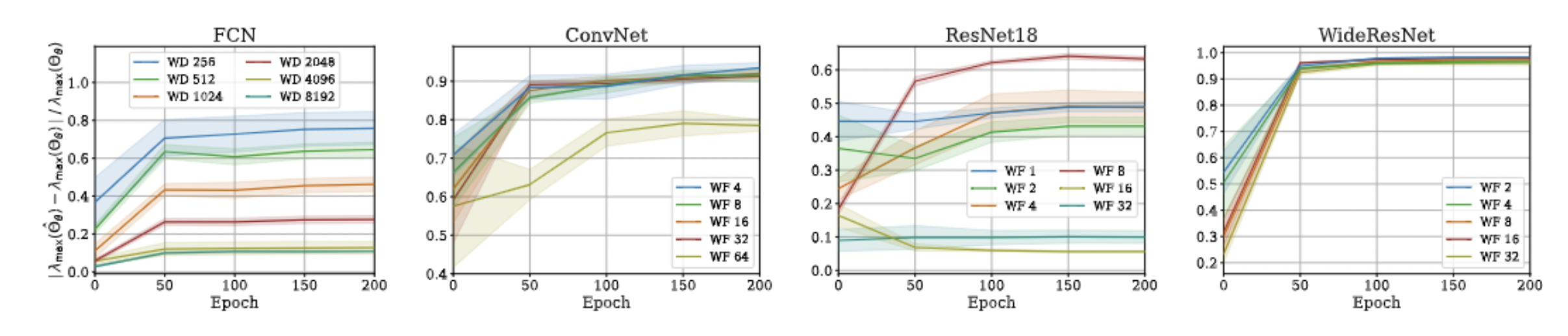
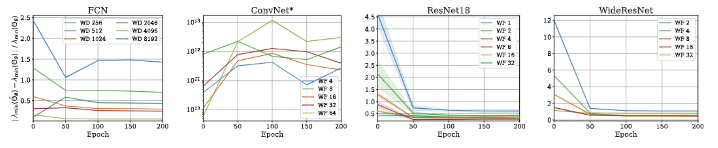
Approximation Error: \(\lambda_{\max}\)
\Large\dfrac{| \lambda_{max}(\Theta_\theta(x_1, x_2)) - \lambda_{max}(\hat\Theta_\theta(x_1, x_2) \times I_{O})| }{\lambda_{max}(\Theta_\theta(x_1, x_2))} = \mathcal O \Big(\dfrac{1}{\sqrt{n}} \Big)
-
Theorem 2: Consider a fully-connected neural network whose parameters are initialized according to Standard Parameterization (fan_in). The following equality holds w.h.p over random initialization:
where \(n\) denotes the width of network.
- Proof idea: The nominator is bounded by \(||D(x_1,x_2)||_F = \mathcal O(\sqrt{n})\) and the denominator's diagonal elements are \(\Theta(n)\), both w.h.p. over random init.
Approximation Error: \(\lambda_{\max}\)
Approximation Error:
Kernel Regression
- Note that pNTK is a scalar-valued kernel, but the eNTK is a matrix-valued kernel!
- Intuitively, one might expect that they can not be used in the same context for kernel regression.
- But, there's a work-around, as this is a well known problem:
Approximation Error:
Kernel Regression
-
Theorem 3: Consider a fully-connected neural network whose parameters are initialized according to Standard Parameterization (fan_in). The following equality holds w.h.p over random initialization:
where \(n\) denotes the width of network.
-
Note: This bound will not hold if there is any regularization (ridge) in the kernel regression! :(
||\hat f^{lin}(x) - f^{lin}(x) ||_2 = \mathcal O \Big(\dfrac{1}{\sqrt{n}} \Big)
Approximation Error:
Kernel Regression
\alpha = {\Big( \frac{1}{n} \Theta(\mathcal X, \mathcal X) \Big)}^{-1} \mathcal Y
\alpha' = {\Big( \frac{1}{n} \hat\Theta(\mathcal X, \mathcal X) \otimes I_O \Big)}^{-1} \mathcal Y
- Using the fact that \( {\hat M}^{-1} - M^{-1} = -{\hat M}^{-1} ( \hat M - M) M^{-1}\):
||\alpha - \alpha'|| \le \dfrac{1}{\lambda^2 n} \Big|\Big| \hat\Theta(\mathcal X, \mathcal X) \otimes I_O - \Theta(\mathcal X, \mathcal X) \Big|\Big| ||\mathcal Y||
- Proof Idea: Kernel regression without regularization is scale-invariant. To bound the inverses, define:
- Using the previous bounds on \( D(x_1, x_2) \), we can conclude the proof.
Approximation Error:
Kernel Regression
Pseudo-NTK: Speed-Up
Extending the Proof to
Other Settings
- Most initialization methods result in subgaussian independent weight scalars. Hence, one can accordingly use the Hanson-Wright inequality.
- We can plug in different activation functions as long as we can prove a high probability bound on dot-product of post-activations growing linearly with width.
- Thanks to Greg Yang's Tensor Programs, it's easy to see that the recursive definition of eNTK applies to most of the architectures.
A Note On The Current Version of The Manusript
Application: "Look-Ahead" Deep Active Learning
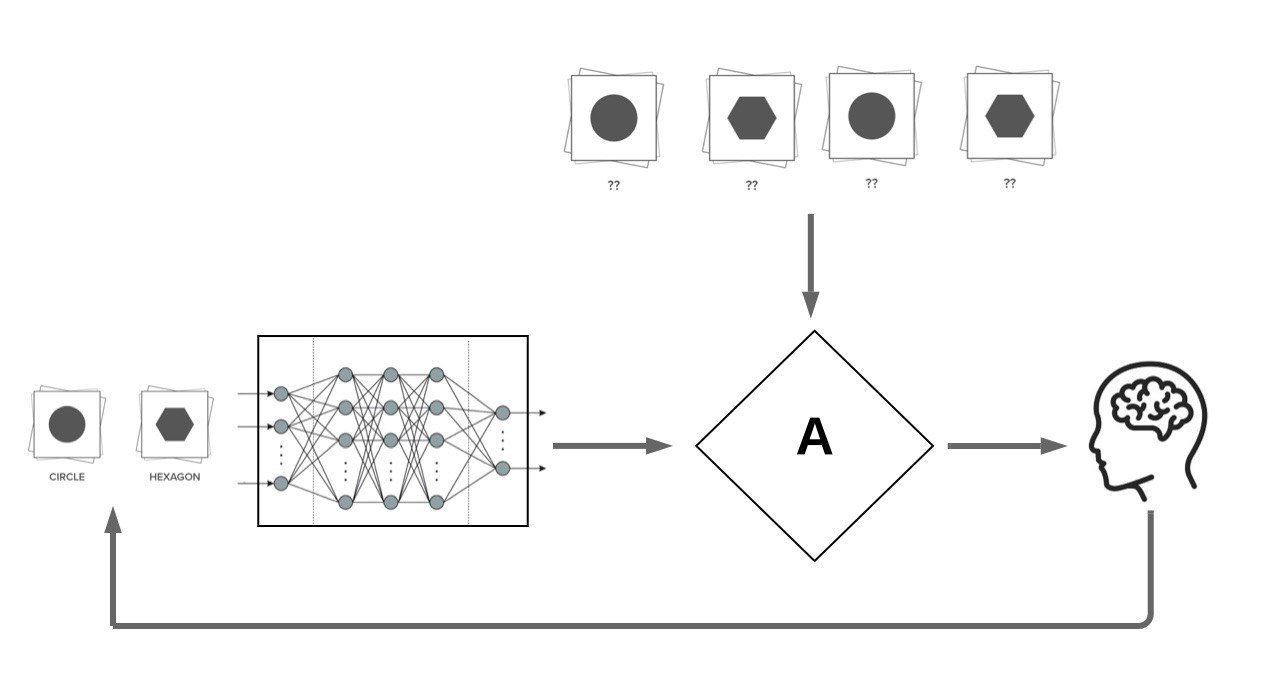
Active learning: reducing the required amount of labelled data in training ML models through allowing the model to "actively request for annotation of specific datapoints".
We focus on Pool Based Active Learning:
x^* = \argmax_{x \in \mathcal{U}}{A \left(x, f_{\mathcal{L}}, \mathcal{L}, \mathcal{U}\right)}
f_{\mathcal{L}}
\mathcal{U}
\mathcal{L}
x^*
x
(x^*, y^*)
AL Acquisition Functions
Most proposed acquisition functions in deep active learning can be categorized to two branches:
- Uncertainty Based: Maximum Entropy, BALD
- Representation-Based: BADGE, LL4AL
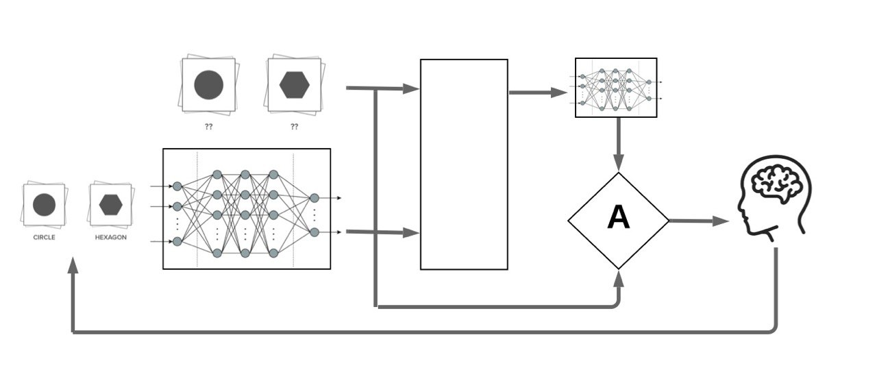
Our Motivation: Making Look-Ahead acquisition functions feasible in deep active learning:
x
f_{\mathcal{L} \, \cup \, (x, \hat{y})}
\mathcal{L}
f_{\mathcal{L}}
x^*
(x^*, y^*)
Retraining
Engine
\mathcal{U}
Contributions
-
Problem: Retraining the neural network with every unlabelled datapoint in the pool using SGD is practically infeasible.
-
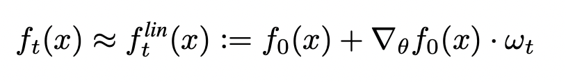
Solution: We propose to use a proxy model based on the first-order Taylor expansion of the trained model to approximate this retraining.
-
Contributions:
- We prove that this approximation is asymptotically exact for ultra wide networks.
- Our method achieves similar or improved performance than best prior pool-based AL methods on several datasets.
-
Our proxy model can be used to perform fast Sequential Active Learning (no SGD needed)!
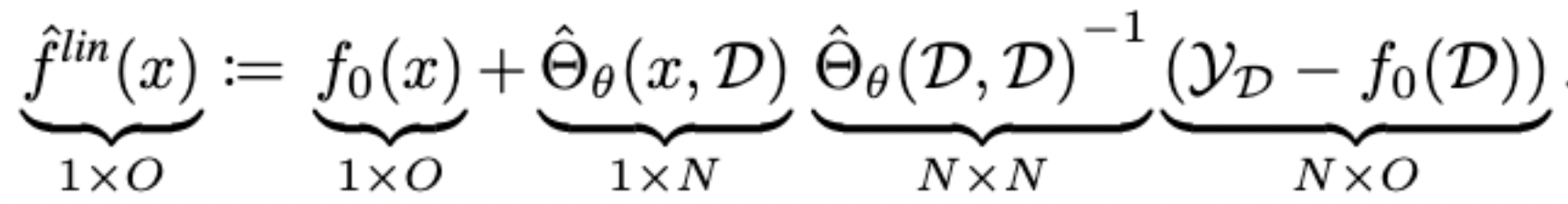
- Idea: approximate the retrained neural network on a new datapoint ( ) using the first-order taylor expansion of the network around the current model.
f_{\mathcal{L} \, \cup \, (x, \hat{y})}
f_{\mathcal{L}}
f_{\mathcal{L}^+}(x)
\approx f^\textit{lin}_{\mathcal{L}^+}(x)
=
f_\mathcal{L}(x) + \Theta_{\mathcal{L}}(x, {\color{blue}{\mathcal{X}}}^{\color{orange}{+}}){\Theta_{\mathcal{L}}({\color{blue}{\mathcal{X}}}^{\color{orange}{+}}, {\color{blue}{\mathcal{X}}}^{\color{orange}{+}})}^{-1} \left (\mathcal{Y}^+ - f_\mathcal{L}(\mathcal{X}^+) \right )
+
-1
-
(
)
\times
f^\textit{lin}_{\mathcal{L}^+}(x) =
- Intuitively, as adding one data-point will most likely not result in drastic changes in weights, using the first-order Taylor expansion should be a good proxy!
Approximation of Retraining
Approximation of Retraining
-
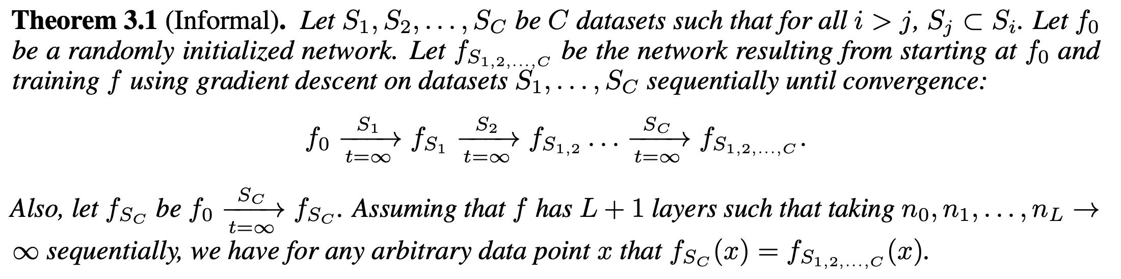
We prove that this approximation is asymptotically exact for ultra wide networks and is empirically comparable to SGD for finite width networks.
- Proof idea: Induction over size of dataset, starting from \(f_0 \) and adding datapoints sequentially.
Approximation of Retraining
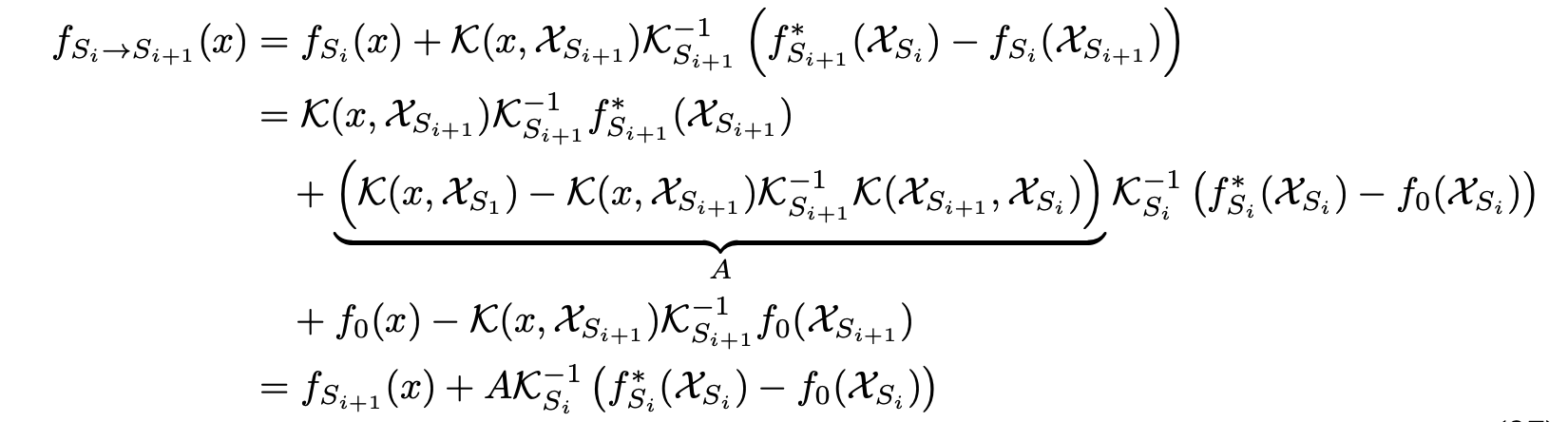
- Based case is trivial. For the transition case, we have:
- \(f_{S_i \to S_{i+1}}(x) \): Function resulting from training with initialization set to \(f_{S_i}\) and training on \(S_{i+1}\) until convergence.
Approximation of Retraining
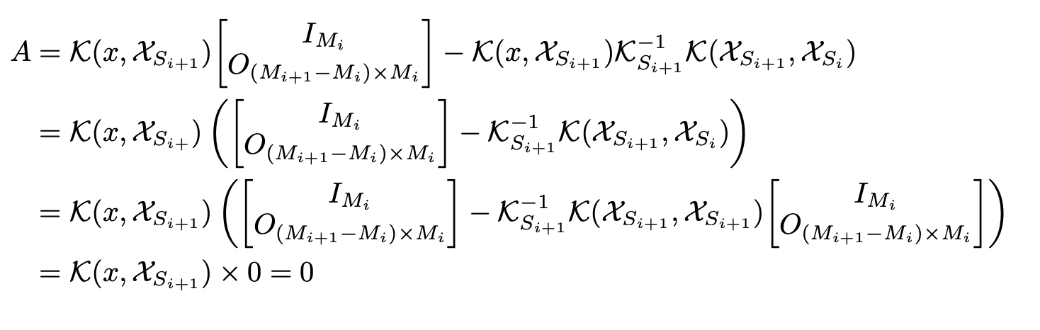
- We can see that \(A\) is equal to zero:
and hence, the induction step holds!
Look-Ahead Active Learning
- We employ the proposed retraining approximation in a well-suited acquisition function which we call the Most Likely Model Output Change (MLMOC):
A_\textit{MLMOC}(x', f_{\mathcal L}, \mathcal{L}_t,\, \mathcal{U}_t)
\vcentcolon=
\sum_{x \in \mathcal{U}} \lVert f_{\mathcal L}(x) - f^\textit{lin}_{\mathcal L^+}(x)) \rVert_2
-
Although our experiments in the pool-based AL setup were all done using MLMOC, the proposed retraining approximation is general.
- We hope that this enables new directions in deep active learning using the look-ahead criteria.
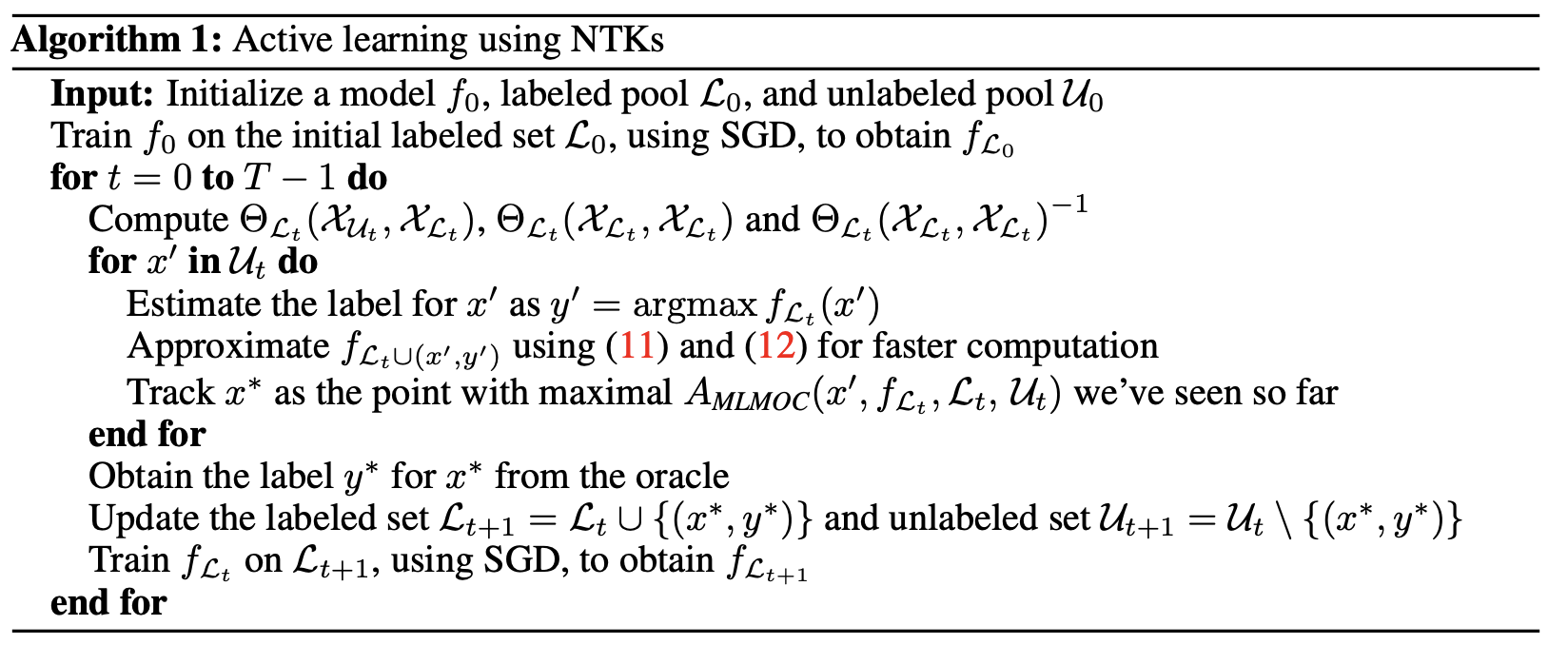
Final Algorithm
Experiments
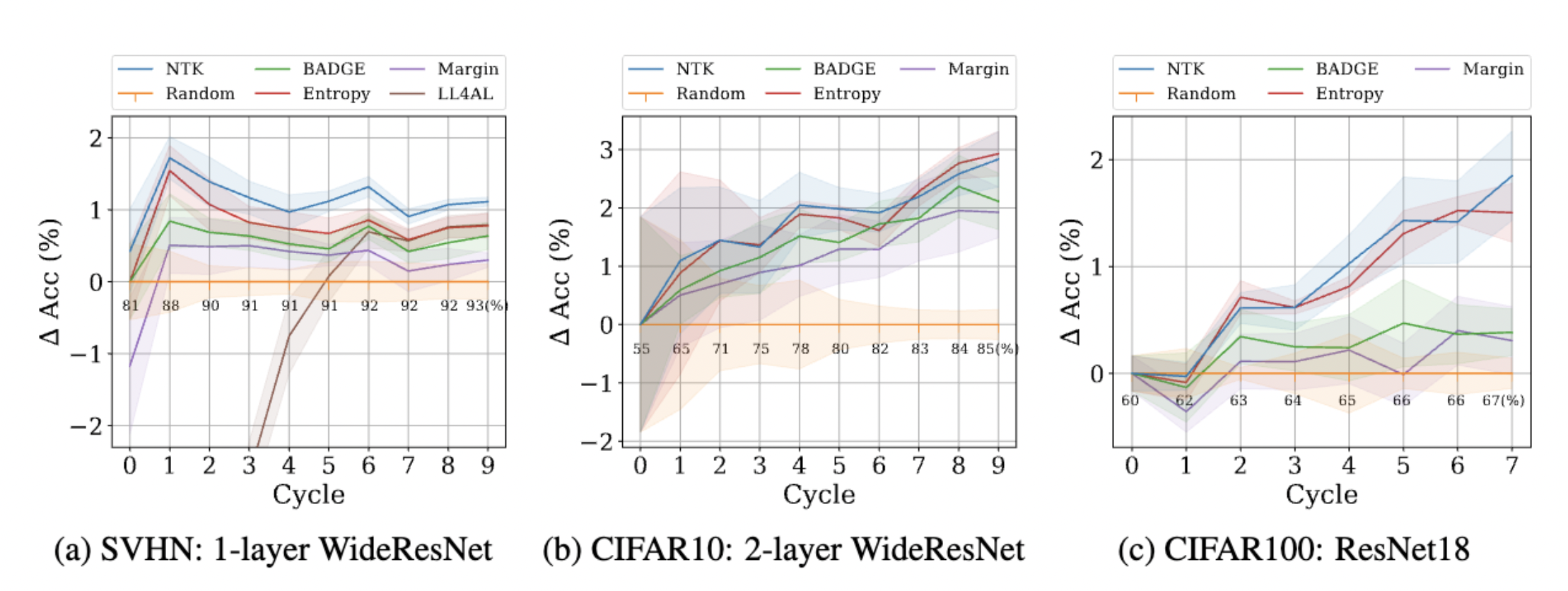
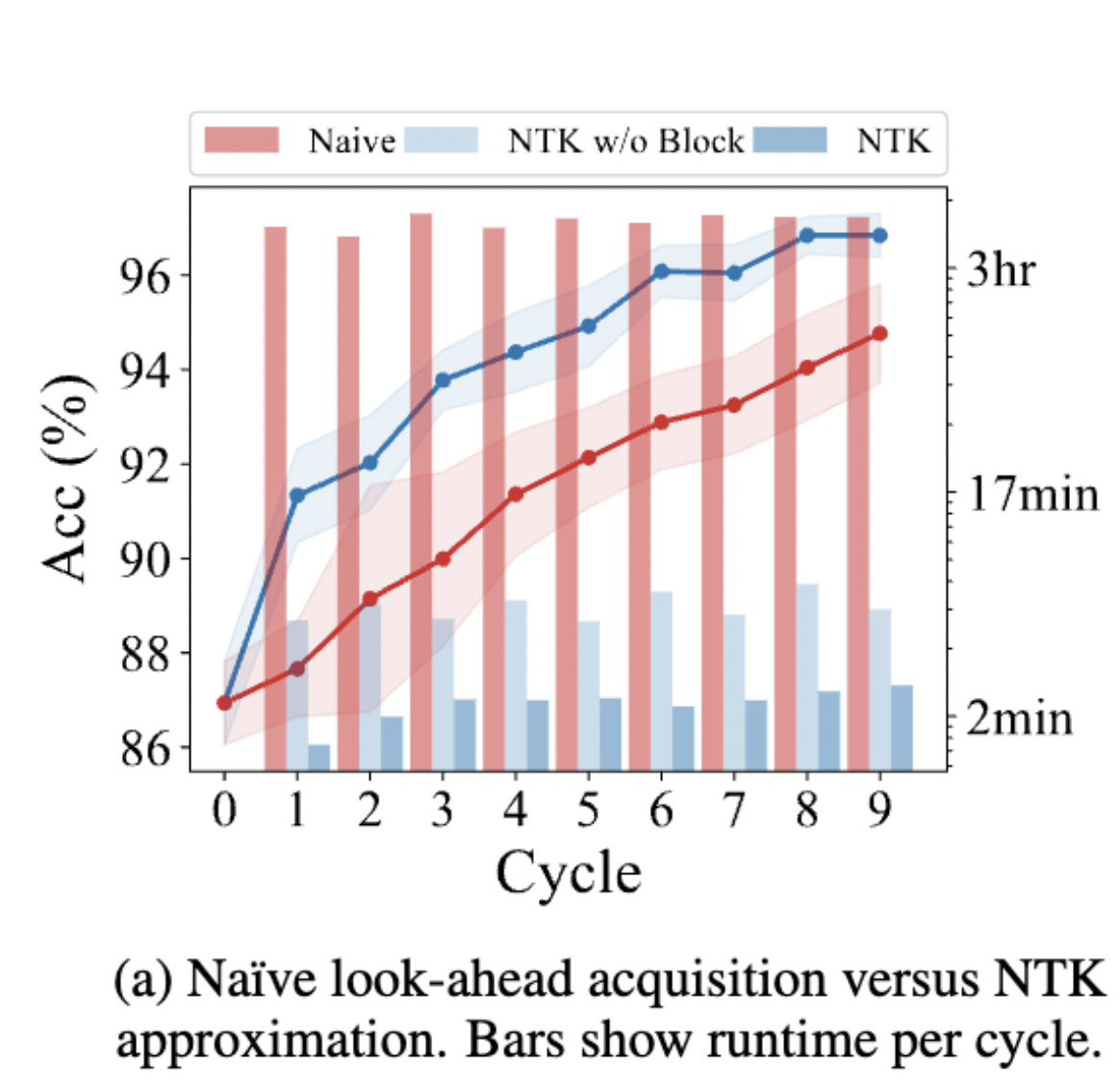
Retraining Time: The proposed retraining approximation is much faster than SGD.
Experiments: The proposed querying strategy attains similar or better performance than best prior pool-based AL methods on several datasets.
Application: Trace of Hessian
\begin{aligned}
\text{Tr} (\nabla_\theta L(f_\theta))
&= \text{Tr} \Big( {\nabla_\theta f_\theta}^\top \times \nabla^2_{f_\theta} L(f_\theta) \times \nabla_\theta f_\theta \Big) \\
&= \text{Tr} \Big( \nabla_\theta f_\theta \times {\nabla_\theta f_\theta}^\top \times \nabla^2_{f_\theta} L(f_\theta) \Big) \\
&= \text{Tr} \Big( \Theta(x, x) \times c \, I_O \Big) \\
&\approx \hat\Theta(x, x) \times c
\end{aligned}
- Pseudo-NTK can be used to approximate the trace of hessian of the loss function. For MSE Loss:
- For Cross Entropy loss, the hessian of loss function with respect to the NN function is not diagonal, but we're still trying to find a work-around.
Thank You! Questions?


Active Learning NTKs on arXiv
Pseudo-NTK on arXiv
brain_march_23
By Amin Mohamadi


