
Amrutha
Course Content Developer for Deep Learning course by Professor Mitesh Khapra. Offered by IIT Madras Online degree - Programming and Data Science.
Machine Learning Techniques
Class: sklearn.linear_model.RidgeClassifier
Some Parameters:
Predict confidence scores for samples. |
|
densify() |
Convert coefficient matrix to dense array format. |
fit(X, y[, coef_init, intercept_init, …]) |
Fit linear model with Stochastic Gradient Descent. |
get_params([deep]) |
Get parameters for this estimator. |
partial_fit(X, y[, classes, sample_weight]) |
Perform one epoch of stochastic gradient descent on given samples. |
predict(X) |
Predict class labels for samples in X. |
Log of probability estimates. |
|
Probability estimates. |
|
score(X, y[, sample_weight]) |
Return the mean accuracy on the given test data and labels. |
set_params(**params) |
Set the parameters of this estimator. |
sparsify() |
Convert coefficient matrix to sparse format. |
Some common methods for all classifiers
Class: sklearn.linear_model.LogisticRegression
Some Parameters:
'none' - no penalty is added
'l2' - add a L2 penalty term and it is the default choice
'l1' - add a L1 penalty term
'elasticnet' - both L1 and L2 penalty terms are added
solver (default = 'lbfgs')
'liblinear' - uses a coordinate descent (CD) algorithm
'lbfgs' - an optimizer in the family of quasi-Newton methods.
'newton-cg', 'sag', 'saga'
SGDClassifier(loss='log')
LogisticRegression(solver='sgd')
SGDClassifier(loss='hinge')
Linear Support vector machine
Class: sklearn.linear_model.SGDClassifier
This estimator implements regularized linear models with SGD.
The gradient of the loss is estimated each sample at a time and the model is updated along the way with a decreasing learning rate.
Some parameters
penalty - 'l2’, ‘l1’, ‘elasticnet’ (default = 'l2')
loss (default = 'hinge')
'hinge' - (soft-margin) linear Support Vector Machine,
'modified_huber' - smoothed hinge loss brings tolerance to outliers as well as probability estimates
'log' - logistic regression
'squared_hinge' - like hinge but is quadratically penalized
'perceptron' - linear loss used by the perceptron algorithm
regression losses - ‘squared_error’, ‘huber’, ‘epsilon_insensitive’, or ‘squared_epsilon_insensitive’
alpha (default = 0.0001)
constant that multiplies the regularization term.
fit_intercept (default = True)
If False, the data is assumed to be already centered.
max_iter (default = 1000)
maximum number of passes over the training data (aka epochs).
learning_rate (default = ’optimal’)
‘constant’: eta = eta0 (default eta0=0.0, initial learning rate)
‘optimal’: eta = 1.0 / (alpha * (t + t0)) where t0 is chosen by a heuristic proposed by Leon Bottou.
‘invscaling’: eta = eta0 / pow(t, power_t)
‘adaptive’: eta = eta0 , as long as the training keeps decreasing. Each time n_iter_no_change consecutive epochs fail to decrease the training loss by tol or fail to increase validation score by tol if early_stopping is True, the current learning rate is divided by 5.
tol (default = 1e-3)
stopping criterion.
If it is not None, training will stop when (loss > best_loss - tol) for n_iter_no_change consecutive epochs.
Convergence is checked against the training loss or the validation loss depending on the early_stopping parameter.
early_stopping (default = False)
to terminate training when validation score is not improving.
If set to True, it will automatically set aside a stratified fraction of training data as validation and terminate training when validation score returned by the score method is not improving by at least tol for n_iter_no_change consecutive epochs
validation_fraction (default = 0.1)
proportion of training data to set aside as validation set for early stopping . Must be between 0 and 1.
Only used if early_stopping
n_iter_no_change (default = 5)
Number of iterations with no improvement to wait before stopping fitting.
Convergence is checked against the training loss or the validation loss depending on the early_stopping
class_weight (default = None) {class_label: weight} or “balanced”,
The “balanced” mode uses the values of y to automatically adjust weights inversely proportional to class frequencies in the input data as n_samples / (n_classes * np.bincount(y)).
Preset for the class_weight fit parameter. Weights associated with classes. If not given, all classes are supposed to have weight one.
It is a simple classification algorithm suitable for large-scale learning.
Class: sklearn.linear_model.Perceptron
Some Parameters:
penalty - 'l2’, ‘l1’, ‘elasticnet’ (default = 'l2')
alpha - (default = 0.0001)
l1_ratio - (default = 0.15)
fit_intercept - (default = True)
max_iter - (default = 1000)
tol - (default = 1e-3)
eta0 - (default = 1)
early_stopping - (default = False)
validation_fraction - (default = 0.1)
n_iter_no_change - (default = 5)
scikit-learn implements two different nearest neighbors classifiers.| KNeighborsClassifier | RadiusNeighborsClassifier |
|---|---|
| implements learning based on the k nearest neighbors of each query point, where k is an integer value specified by the user. | implements learning based on the number of neighbors within a fixed radius r of each training point, where r is a floating-point value specified by the user. |
| most commonly used technique choice of the value k is highly data-dependent |
used in cases where the data is not uniformly sampled |
| larger k suppresses the effects of noise, but makes the classification boundaries less distinct. | user specifies a fixed radius r, such that points in sparser neighborhoods use fewer nearest neighbors for the classification |
Class: sklearn.neighbors.KNeighborsClassifier
Some Parameters
Class: sklearn.neighbors.RadiusNeighborsClassifier
Some Parameters
Range of parameter space to use by default for radius_neighbors queries
weights (‘uniform’, ‘distance’, [callable], default = ’uniform')
algorithm (‘ball_tree’, ‘kd_tree’, ‘brute’, ‘auto’, default = 'auto'
leaf_size (default = 30)
p (default = 2)
metric (default = ’minkowski’)
Distance metric to use for the tree.
Multiclass classification
(sklearn.multiclass)
Multilabel classification
(sklearn.multioutput)
problem types
meta-estimators
OneVsOneClassifier
OneVsRestClassifier
OutputCodeClassifier
MultiOutputClassifier
ClassifierChain
sklearn.utils.multiclass.type_of_target
determines the type of data indicated by the target.
Parameters : y (array-like), Returns : target_type (string)
| target_type | y |
|---|---|
| 'continuous' | array-like of floats that are not all integers and is 1d or a column vector. |
| 'continuous-multioutput' | 2d array of floats that are not all integers, and both dimensions are of size > 1. |
| ‘binary’ | contains <= 2 discrete values and is 1d or a column vector. |
| ‘multiclass’ | contains more than two discrete values, is not a sequence of sequences, and is 1d or a column vector. |
| ‘multiclass-multioutput’ | 2d array that contains more than two discrete values, is not a sequence of sequences, and both dimensions are of size > 1. |
| ‘unknown’ | array-like but none of the above, such as a 3d array, sequence of sequences, or an array of non-sequence objects. |
>>> from sklearn.utils.multiclass import type_of_target
>>> import numpy as np
>>> type_of_target([0.1, 0.6])
'continuous'
>>> type_of_target([1, -1, -1, 1])
'binary'
>>> type_of_target(['a', 'b', 'a'])
'binary'
>>> type_of_target([1.0, 2.0])
'binary'>>> type_of_target([1, 0, 2])
'multiclass'
>>> type_of_target([1.0, 0.0, 3.0])
'multiclass'
>>> type_of_target(['a', 'b', 'c'])
'multiclass'>>> type_of_target(np.array([[1, 2], [3, 1]]))
'multiclass-multioutput'>>> type_of_target(np.array([[1.5, 2.0], [3.0, 1.6]]))
'continuous-multioutput'continuous-multioutput
continuous
binary
multiclass
multiclass-multioutput
Constructs one classifier per pair of classes.
At prediction time, the class which received the most votes is selected. In the event of a tie, it selects the class with the highest aggregate classification confidence by summing over the pair-wise classification confidence levels computed by the underlying binary classifiers.
classifiers needed = \(\dfrac{n_{classes}\times(n_{classes} - 1)}{2} \)
slower than one-vs-the-rest, due to its \(O(n_{classes}^2)\) complexity.
advantage : for kernel algorithms which don’t scale well
| target_type | y |
|---|---|
| ‘multilabel-indicator’ | label indicator matrix, an array of two dimensions with at least two columns, and at most 2 unique values. |
type_of_target(np.array([[0, 1], [1, 1]]))
'multilabel-indicator'
>>> type_of_target([[1, 2]])
'multilabel-indicator'
multilabel-indicator
| MultiOutputClassifier | ClassifierChain |
|---|---|
| Strategy consists of fitting one classifier per target. | Way of combining a number of binary classifiers into a single multi-label model that is capable of exploiting correlations among targets. |
| Allows multiple target variable classifications. Able to estimate a series of target functions that are trained on a single predictor matrix to predict a series of responses. |
For a multi-label classification problem with N classes, N binary classifiers are assigned an integer between 0 and N-1. These integers define the order of models in the chain. |
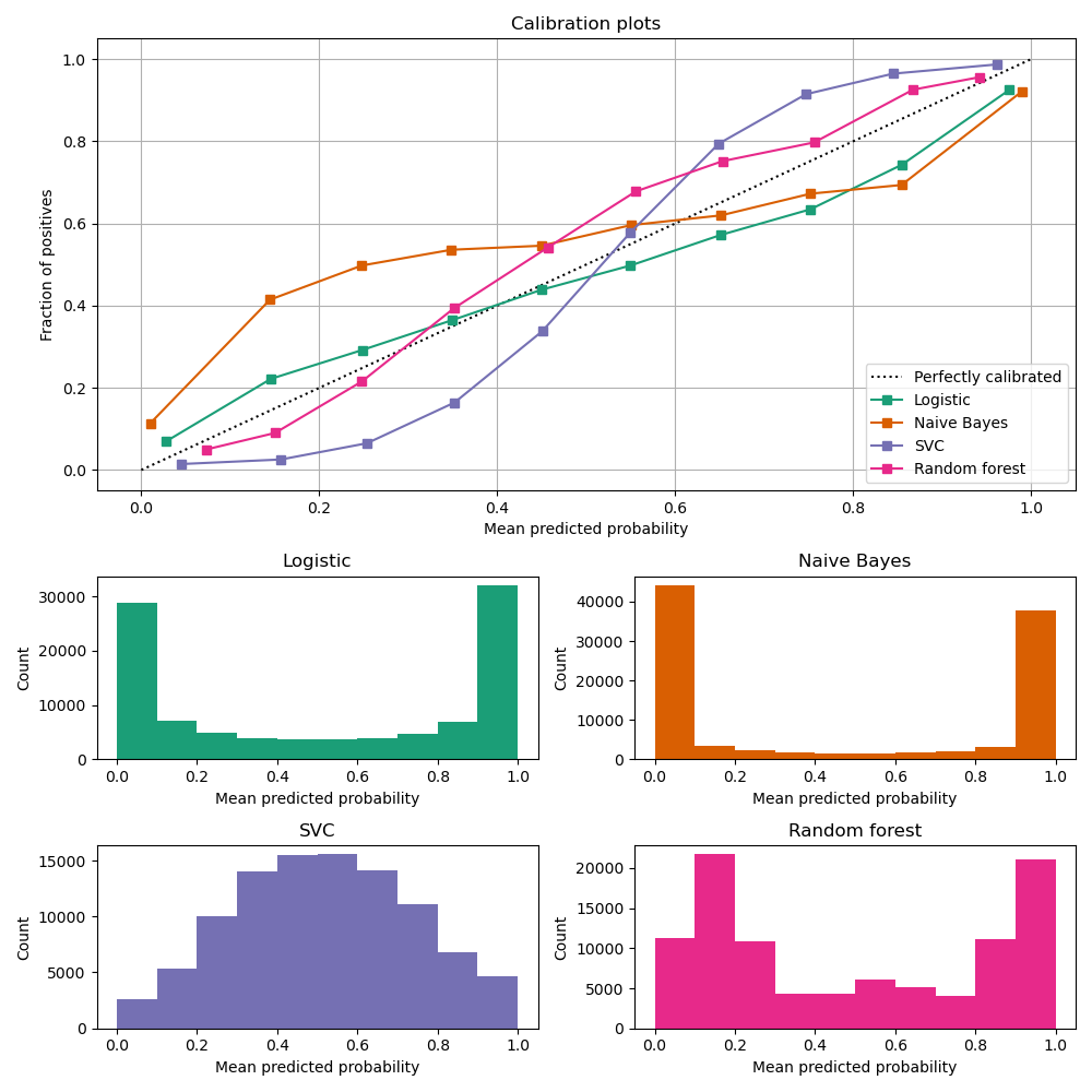
Calibration curves
compare how well the probabilistic predictions of a binary classifier are calibrated.
plots the true frequency of the positive label against its predicted probability, for binned predictions.
x axis : average predicted probability in each bin
y axis : fraction of positives, i.e. the proportion of samples whose class is the positive class (in each bin).
Image Source: https://scikit-learn.org/stable/modules/calibration.html
LogisticRegression returns well calibrated predictions by default as it directly optimizes Log loss.
GaussianNB tends to push probabilities to 0 or 1.
RandomForestClassifier peaks at approximately 0.2 and 0.9 probability, while probabilities close to 0 or 1 are very rare.
LinearSVC focus on difficult to classify samples that are close to the decision boundary (the support vectors).
ensemble = True
ensemble = False
Model selection for classification
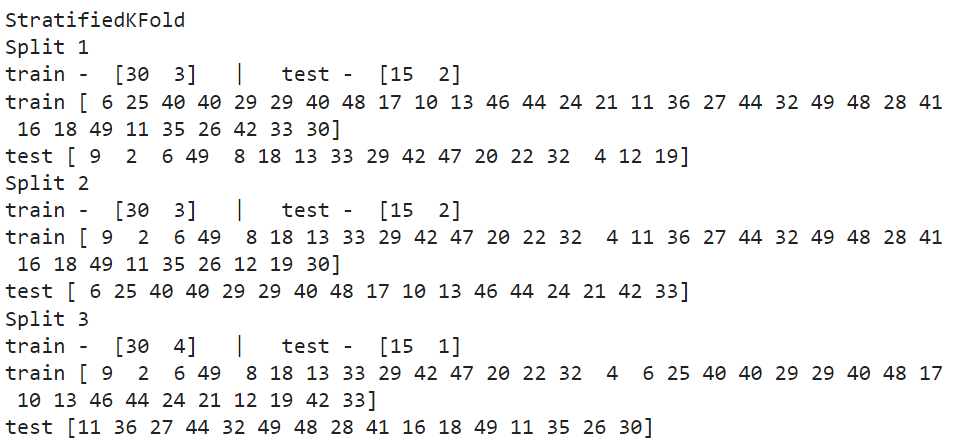
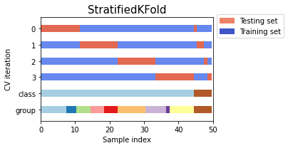
Class: sklearn.model_selection.StratifiedKFold
Some Parameters:
n_splits (default = 5)
Number of folds. Must be at least 2.
shuffle (default = False)
to shuffle or not to shuffle each class’s samples before splitting into batches.
samples within each split will not be shuffled.
random_state RandomState instance or None, (default=None)
set random_state when shuffle = True because it affects the ordering of the indices, which controls the randomness of each fold for each class.
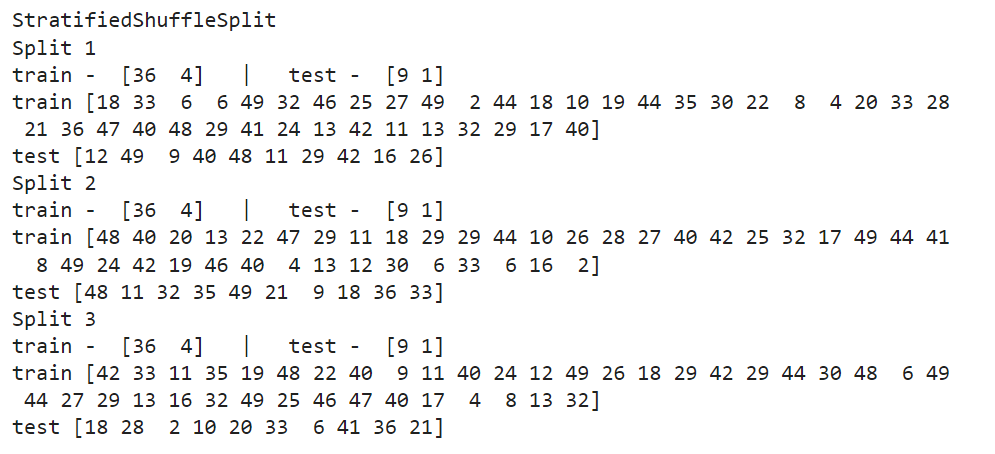
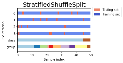
Class: sklearn.model_selection.StratifiedShuffleSplit
Some Parameters:
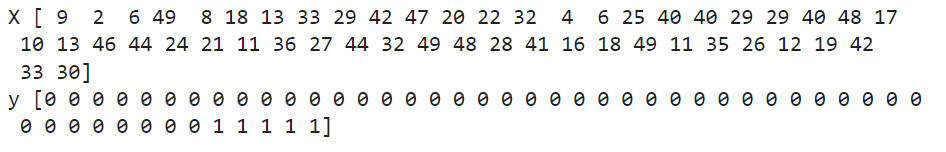
from sklearn.model_selection import StratifiedKFold, StratifiedShuffleSplit
import numpy as np
X, y = np.random.randint(1,50,50), np.hstack(([0] * 45, [1] * 5))
print('X',X)
print('y',y)
skf = StratifiedKFold(n_splits=3)
print('StratifiedKFold')
count = 1
for train, test in skf.split(X, y):
  print('Split', count)
  print('train -  {}   |   test -  {}'.format(np.bincount(y[train]), np.bincount(y[test])))
  print('train',X[train])
  print('test',X[test])
  count+=1
print('StratifiedShuffleSplit')
sss = StratifiedShuffleSplit(n_splits=3, test_size=0.2, random_state=0)
count = 1
for train_index, test_index in sss.split(X, y):
  print('Split', count)
  print('train -  {}   |   test -  {}'.format(np.bincount(y[train_index]), np.bincount(y[test_index])))
  print('train',X[train_index])
  print('test',X[test_index])
  count+=1
Example to compare StratifiedKFold and StratifiedShuffleSplit
Output:
Class: sklearn.linear_model.LogisticRegressionCV
Some Parameters:
'Cs' (default = 10)
Each of the values in Cs describes the inverse of regularization strength.
If int, then a grid of values = logarithmic scale between \(1e^{-4}\) & \(1e^4\).
'cv' (default = None)
The default cross-validation generator used is Stratified K-Folds.
If an integer is provided, then it is the number of folds used.
scoring (default = None)
A string or scorer(estimator, X, y) . (default scoring option used is ‘accuracy’).
penalty (‘l1’, ‘l2’, ‘elasticnet’, default=‘l2’)
refit (default = True)
If set to True, the scores are averaged across all folds, and the coefs and the C that corresponds to the best score is taken, and a final refit is done using these parameters.
Otherwise the coefs, intercepts and C that correspond to the best scores across folds are averaged.
l1_ratios list of float, (default = None)
The list of Elastic-Net mixing parameter, with 0 <= l1_ratio <= 1 .
Only used if penalty='elasticnet'.
A value of 0 is equivalent to using penalty='l2', while 1 is equivalent to using penalty='l1'.
For 0 < l1_ratio <1 , the penalty is a combination of L1 and L2.
Multiclass classification
Note: The multiclass and multilabel metrics also work for binary classification.
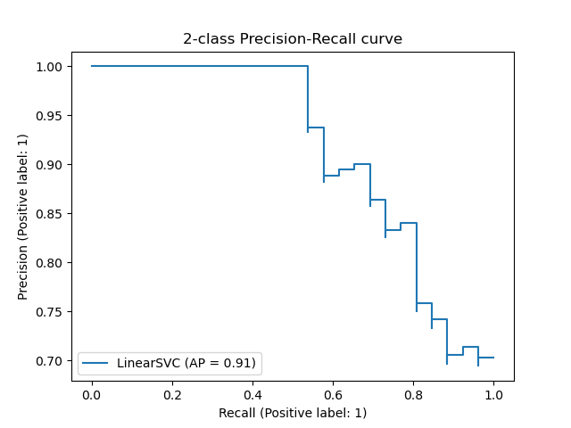
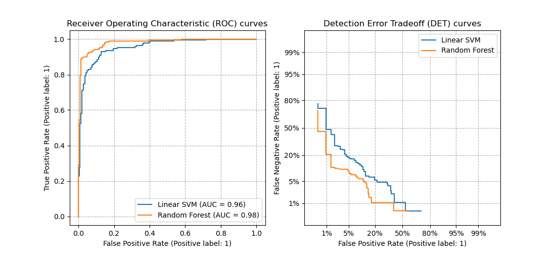
1. sklearn.metrics.precision_recall_curve
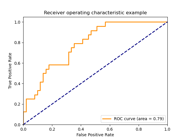
2. sklearn.metrics.roc_curve
3. sklearn.metrics.det_curve
average parameter.
"macro" - calculates the mean of the binary metrics, giving equal weight to each class.
"weighted" - computes the average of binary metrics in which each class’s score is weighted by its presence in the true data sample.
"micro" - gives each sample-class pair an equal contribution to the overall metric (except as a result of sample-weight). (preferred in multilabel settings, including multiclass classification where a majority class is to be ignored.)
"samples" - calculates the metric over the true and predicted classes for each sample in the evaluation data, and returns their (sample_weight-weighted) average.
"None" will return an array with the score for each class.
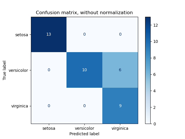
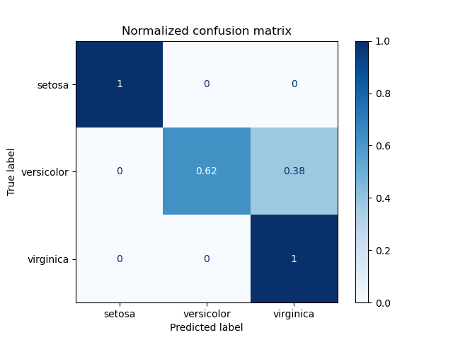
1. sklearn.metrics.confusion_matrix
2. sklearn.metrics.balanced_accuracy_score
3. sklearn.metrics.cohen_kappa_score
4. sklearn.metrics.hinge_loss
5. sklearn.metrics.matthews_corrcoef
6. sklearn.metrics.roc_auc_score
7. sklearn.metrics.top_k_accuracy_score
1. sklearn.metrics.accuracy_score
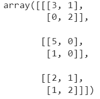
2. sklearn.metrics.multilabel_confusion_matrix
from sklearn.metrics import multilabel_confusion_matrix
y_true = ["cat", "ant", "cat", "cat", "ant", "bird"]
y_pred = ["ant", "ant", "cat", "cat", "ant", "cat"]
multilabel_confusion_matrix(y_true, y_pred,labels=["ant", "bird", "cat"])
3. sklearn.metrics.classification_report
4. sklearn.metrics.zero_one_loss
normalize parameter is True, this function returns the fraction of misclassifications (float), else it returns the number of misclassifications (int).
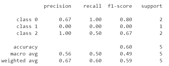
from sklearn.metrics import classification_report
y_true = [0, 1, 2, 2, 0]
y_pred = [0, 0, 2, 1, 0]
target_names = ['class 0', 'class 1', 'class 2']
print(classification_report(y_true, y_pred, target_names=target_names))
4. sklearn.metrics.hamming_loss
5. sklearn.metrics.log_loss
predict_proba method.6. sklearn.metrics.jaccard_score
y_true .7. Precision, recall and F-measures
Note: Best value is 1 and the worst value is 0 for these scores.
sklearn.metrics.precision_score |
computes precision which is intuitively the ability of the classifier not to label as positive a sample that is negative. |
sklearn.metrics.recall_score |
computes recall which is intuitively the ability of the classifier to find all the positive samples. |
sklearn.metrics.f1_score |
computes harmonic mean of precision and recall |
sklearn.metrics.fbeta_score |
computes weighted harmonic mean of precision and recall |
sklearn.metrics.average_precision_score |
computes the average precision from prediction scores (this score does not supports multiclass) |
8. sklearn.metrics.precision_recall_fscore_support
By Amrutha


