Quantum Monte Carlo approaches for strongly correlated systems
Variational Monte Carlo
Stochastic multireference perturbation theory
Auxiliary field QMC


Outline
- Sampling and the sign problem in AFQMC
- Reducing noise using selected CI wave functions
- Benchmark results
- Jastrow symmetry projected states in VMC
- Auxiliary field QMC
- Variational MC
- Use in projection QMC
A different take on projection QMC
Projection QMC methods:
e^{-\tau (\hat{H}-E_0)}|\psi\rangle = c_0|\Psi_0\rangle + c_1 e^{-\Delta E_1\tau}|\Psi_1\rangle+\dots
|\psi\rangle = c_0|\Psi_0\rangle + c_1|\Psi_1\rangle +\dots
- Better \(|\psi\rangle\) approximates \(|\Psi_0\rangle\), faster the convergence with \(\tau\)
E(\tau)=\dfrac{\langle\psi_l|\hat{H}e^{-\tau \hat{H}}|\psi_r\rangle}{\langle\psi_l|e^{-\tau \hat{H}}|\psi_r\rangle}
Mixed energy estimator:
Trial states: Multi-Slater, CCSD, Jastrow, MPS, ...
- Sign problem worsens exponentially with \(\tau\)
Sampling in AFQMC
\hat{H} = \hat{K} + \hat{V} = t_{pr} \hat{a}_{p}^{\dagger}\hat{a}_r + \frac{1}{2}v_{prqs}\hat{a}_{p}^{\dagger}\hat{a}_r\hat{a}_{q}^{\dagger}\hat{a}_{s}
Exponentiating \(\hat{H}\): \([\hat{K}, \hat{V}] \neq 0\)
e^{-\tau\hat{H}}\approx\left(e^{-\frac{\tau}{N}\frac{\hat{K}}{2}}e^{-\frac{\tau}{N}\hat{V}}e^{-\frac{\tau}{N}\frac{\hat{K}}{2}}\right)^N
- Exponentiating \(\hat{K}\): orbital transformation
e^{t_{pr}\hat{a}_p^{\dagger}\hat{a}_r}|\phi\rangle=|\phi'\rangle
where \(|\phi\rangle\) and \(|\phi'\rangle\) are nonorthogonal determinants.
- Exponentiating \(\hat{V} = \frac{1}{2}\sum_{\gamma} \left(L^{\gamma}_{pr}\hat{a}_p^{\dagger}\hat{a}_r\right)^2\):
e^{-\frac{\hat{L}_{\gamma}^2}{2}} = \int \frac{dx_{\gamma}}{\sqrt{2\pi}}\ e^{\frac{-x_{\gamma}^2}{2}}e^{ix_{\gamma}\hat{L}_{\gamma}}
\(x_{\gamma}\): auxiliary field
Motta and Zhang (2017), 1711.02242
(Thouless, 1960)
(Stratonovich, 1957)
E(\tau) = \dfrac{\langle\psi_l|\hat{H}e^{-\tau \hat{H}}|\psi_r\rangle}{\langle\psi_l|e^{-\tau \hat{H}}|\psi_r\rangle} \approx \dfrac{\int\ dX p(X)\langle\psi_l|\hat{H}\hat{\mathcal{B}}(X)|\psi_r\rangle}{\int\ dX p(X)\langle\psi_l|\hat{\mathcal{B}}(X)|\psi_r\rangle}
Sample Gaussian auxiliary fields \(X\), propagate, and measure
E(\tau)\approx\dfrac{\sum_i\langle\psi_l|\hat{H}|\phi_i\rangle}{\sum_i\langle\psi_l|\phi_i\rangle}
CCSD as \(|\psi_r\rangle\): sampling Slater determinants from CCSD
|\psi_r\rangle = \exp\left(t_{ikjl}\hat{a}_i^{\dagger}\hat{a}_k\hat{a}_j^{\dagger}\hat{a}_l\right)\exp\left(t_{ik}\hat{a}_i^{\dagger}\hat{a}_k\right)|\phi_0\rangle
commuting ph excitations \(\rightarrow\) no Trotter error


\((\text{H}_2\text{O})_2\), (16e, 80o)
The sign problem
\text{Var}\left(\dfrac{\overline{N}}{\overline{D}}\right) \approx \dfrac{\text{Var}(\overline{N})}{\overline{D}^2} + \dfrac{\overline{N}^2\text{Var}(\overline{D})}{\overline{D}^4} - 2\dfrac{\overline{N}\text{Cov}(\overline{N},\overline{D})}{\overline{D}^3}
E(\tau)\approx\dfrac{\sum_i\langle\psi_l|\hat{H}|\phi_i\rangle}{\sum_i\langle\psi_l|\phi_i\rangle} = \dfrac{\overline{N}}{\overline{D}}

Contour shift:
e^{-\frac{y^2}{2}} = \int \frac{dx}{\sqrt{2\pi}}\ e^{\frac{-x^2}{2}+ixy}
x\rightarrow x+iy
x_{\gamma} \rightarrow x_{\gamma} + i \sqrt{\tau}\langle\hat{L}_{\gamma}\rangle
In AFQMC:
Baer, Head-Gordon, Neuhauser (1998)


Selected CI trial state as \(|\psi_l\rangle\)
Zero variance principle: If \(|\psi_l\rangle\) is the exact ground state, then \(N\) and \(D\) are perfectly correlated, \(\langle\psi_0|\hat{H}|\phi_i\rangle = E_0 \langle\psi_0|\phi_i\rangle\), and the energy estimator has zero variance.
More accurate \(|\psi_l\rangle\ \rightarrow\ \) higher \(\text{Cov}(N, D)\)
E(\tau)\approx\dfrac{\sum_i\langle\psi_l|\hat{H}|\phi_i\rangle}{\sum_i\langle\psi_l|\phi_i\rangle} = \dfrac{\overline{N}}{\overline{D}}
\text{Var}\left(\dfrac{\overline{N}}{\overline{D}}\right) \approx \dfrac{\text{Var}(\overline{N})}{\overline{D}^2} + \dfrac{\overline{N}^2\text{Var}(\overline{D})}{\overline{D}^4} - 2\dfrac{\overline{N}\text{Cov}(\overline{N},\overline{D})}{\overline{D}^3}

\((\text{H}_2\text{O})_2\), (16e, 80o)
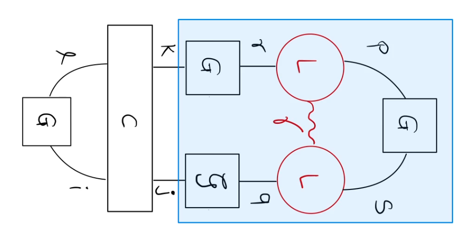
Selected CI local energy algorithm
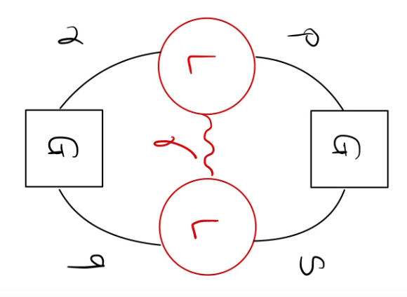
E_L[\phi]=\dfrac{\langle\psi_l|\hat{H}|\phi\rangle}{\langle\psi_l|\phi\rangle},\ \text{two-body part: }\ L^{\gamma}_{pr}L^{\gamma}_{qs}\dfrac{\langle\psi_l|\hat{a}_p^{\dagger}\hat{a}_q^{\dagger}\hat{a}_s\hat{a}_r|\phi\rangle}{\langle\psi_l|\phi\rangle}
If \(|\psi_l\rangle\) is a Slater determinant: \(|\psi_l\rangle = |\phi_0\rangle\)
O(N^4)
If \(|\psi_l\rangle\) is a selected CI wave function: \(|\psi_l\rangle = \sum_i^{N_d} c_i |\phi_i\rangle\)
Naive way: calculating local energy of each Slater determinant as above costs \(O(N_dN^4)\)
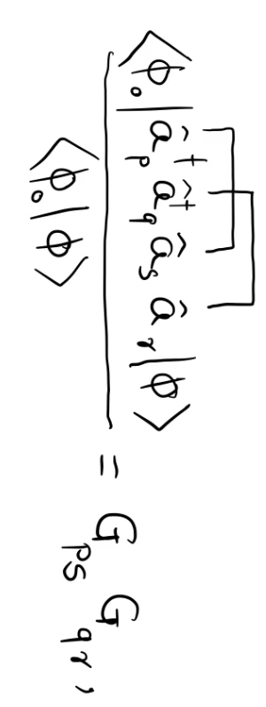
One of the terms:
Consider doubly excited determinants: \(c_{jkil} \hat{a}_j^{\dagger} \hat{a}_k \hat{a}_i^{\dagger} \hat{a}_l |\phi_0\rangle\)

store intermediate
Overall scaling: \(O(N^4 + N_dN)\)
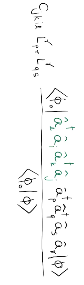
factorizable term

\((\text{H}_2\text{O})_2\), (16e, 80o)
Cyclobutadiene automerization barrier
| Method | DZ (20e, 72o) | TZ (20e, 172o) |
|---|---|---|
| CCSD(T) | 15.8 | 18.2 |
| CCSDT | 7.6 | 10.6 |
| TCCSD (12,12) | - | 9.2 |
| MRCI+Q | - | 9.2 |
| fp-AFQMC | 8.4(4) | 10.2(4) |
kcal/mol
\([\text{Cu}_2\text{O}_2]^{2+}\) isomerization


kcal/mol

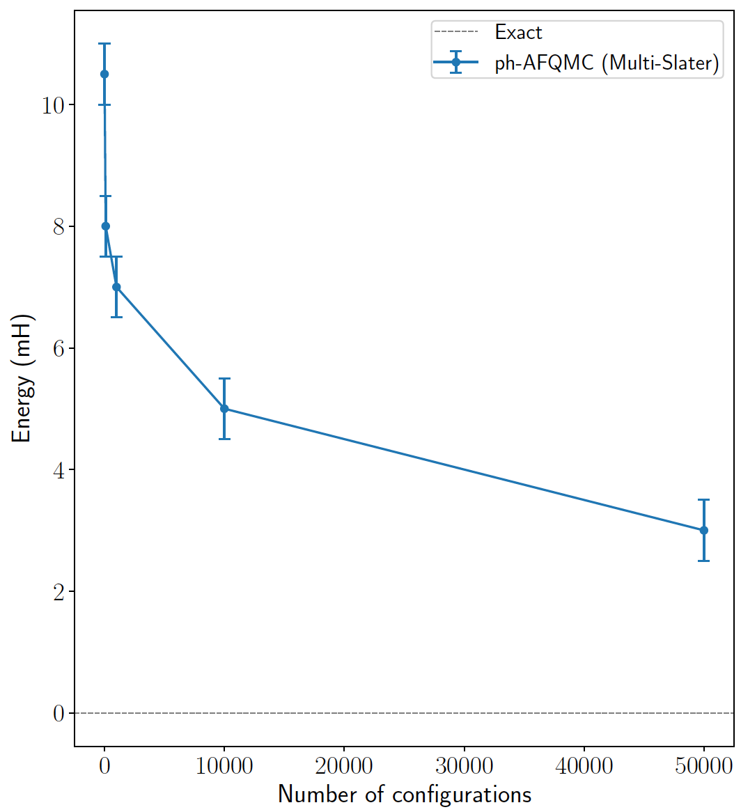
Converging phaseless bias in ph-AFQMC
FeO (22e, 76o)
Symmetry projection in VMC
Symmetry breaking \(\rightarrow\) more variational freedom
Break the symmetry under a projector, to retain good quantum numbers
|\psi\rangle=\hat{P}|\phi\rangle
Projection in VMC by restricting random walk to the symmetry sector
Symmetries: spin, number, complex conjugation, ...
Example: complex conjugation in \(\text{H}_2\) near dissociation

|\text{RHF}\rangle = (a_{1\uparrow}^{\dagger}+a_{2\uparrow}^{\dagger})(a_{1\downarrow}^{\dagger}+a_{2\downarrow}^{\dagger})|0\rangle = (a_{1\uparrow}^{\dagger}a_{1\downarrow}^{\dagger}+a_{1\uparrow}^{\dagger}a_{2\downarrow}^{\dagger}+a_{2\uparrow}^{\dagger}a_{1\downarrow}^{\dagger}+a_{2\uparrow}^{\dagger}a_{2\downarrow}^{\dagger})|0\rangle
|\text{cRHF}\rangle = (e^{i\pi/4}a_{1\uparrow}^{\dagger}+e^{-i\pi/4}a_{2\uparrow}^{\dagger})(e^{i\pi/4}a_{1\downarrow}^{\dagger}+e^{-i\pi/4}a_{2\downarrow}^{\dagger})|0\rangle\\
\quad = (ia_{1\uparrow}^{\dagger}a_{1\downarrow}^{\dagger}+a_{1\uparrow}^{\dagger}a_{2\downarrow}^{\dagger}+a_{2\uparrow}^{\dagger}a_{1\downarrow}^{\dagger}-ia_{2\uparrow}^{\dagger}a_{2\downarrow}^{\dagger})|0\rangle
\hat{K}|\text{cRHF}\rangle = (a_{1\uparrow}^{\dagger}a_{2\downarrow}^{\dagger}+a_{2\uparrow}^{\dagger}a_{1\downarrow}^{\dagger})|0\rangle

\hat{P}\hat{\mathcal{J}}|\psi\rangle = \hat{P}\exp\left(\sum_{p\sigma,q\gamma} v_{p\sigma,q\gamma}\hat{n}_{p\sigma}\hat{n}_{q\gamma}\right)|\psi\rangle
Jastrow symmetry projected state:
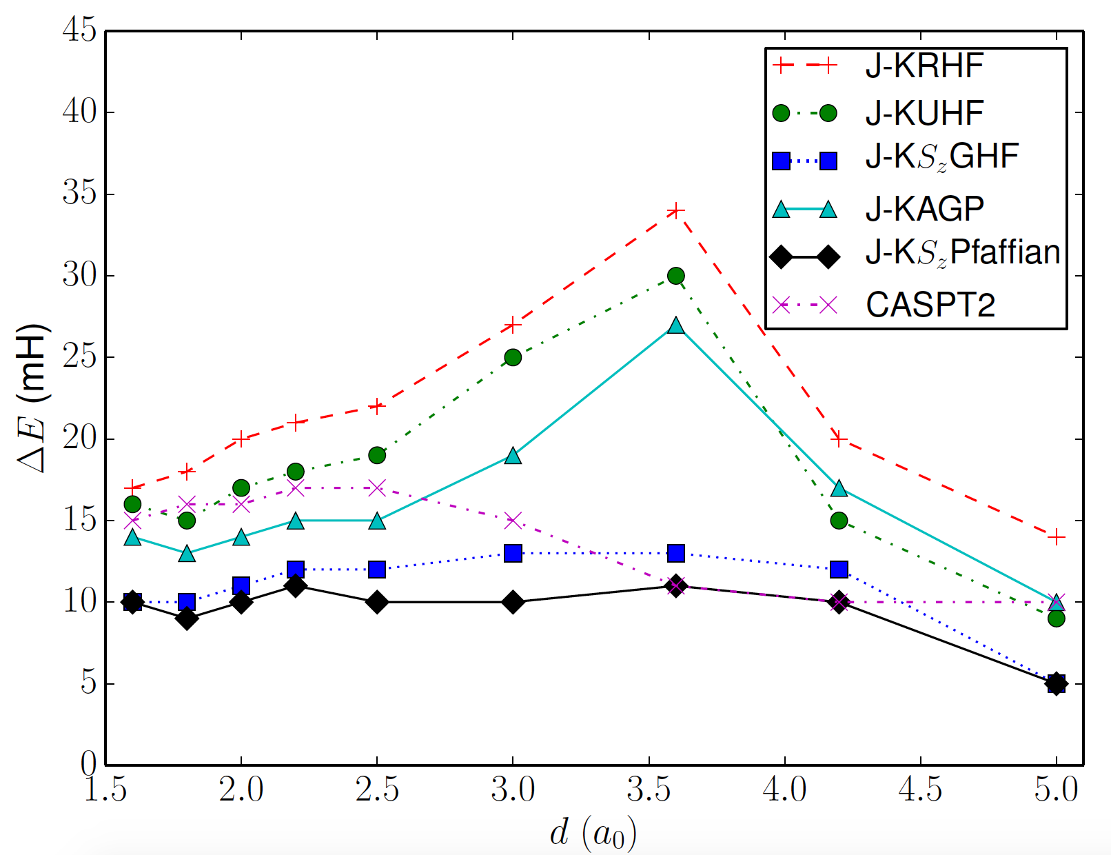
\(\text{N}_2\)
| d (Bohr) | Exact (DMRG) | Jastrow-KS_zPfaffian | Green's function MC |
| 1.6 | -0.5344 | -0.5337 | -0.5342 |
| 1.8 | -0.5408 | -0.5400 | -0.5406 |
| 2.5 | -0.5187 | -0.5180 | -0.5185 |
H\( _{50} \) linear chain (50e, 50o)
| U | Benchmark energy | Jastrow- KS_zGHF |
Green's function MC |
| 2 | -1.1962 | -1.1920 | -1.1939 |
| 4 | -0.8620 | -0.8566 | -0.8598 |
| 8 | -0.5237 | -0.5183 | -0.5221 |
2D Hubbard: 98 sites (half filling)
Hartree/particle
Future directions
- Properties and excited states
- Importance sampling and constraints in AFQMC, hybrid MD-MC
- Variational CCSD, other wave functions like MPS, Jastrow in AFQMC
- Spin liquid states in iridates using VMC
Thank you!
afqmc_vmc
By Ankit Mahajan


