














Andreas Park PRO
Professor of Finance at UofT
Katya Malinova and Andreas Park
Some Motivation
Basic Idea
Key Components
Liquidity Supply and Demand in an Automated Market Maker
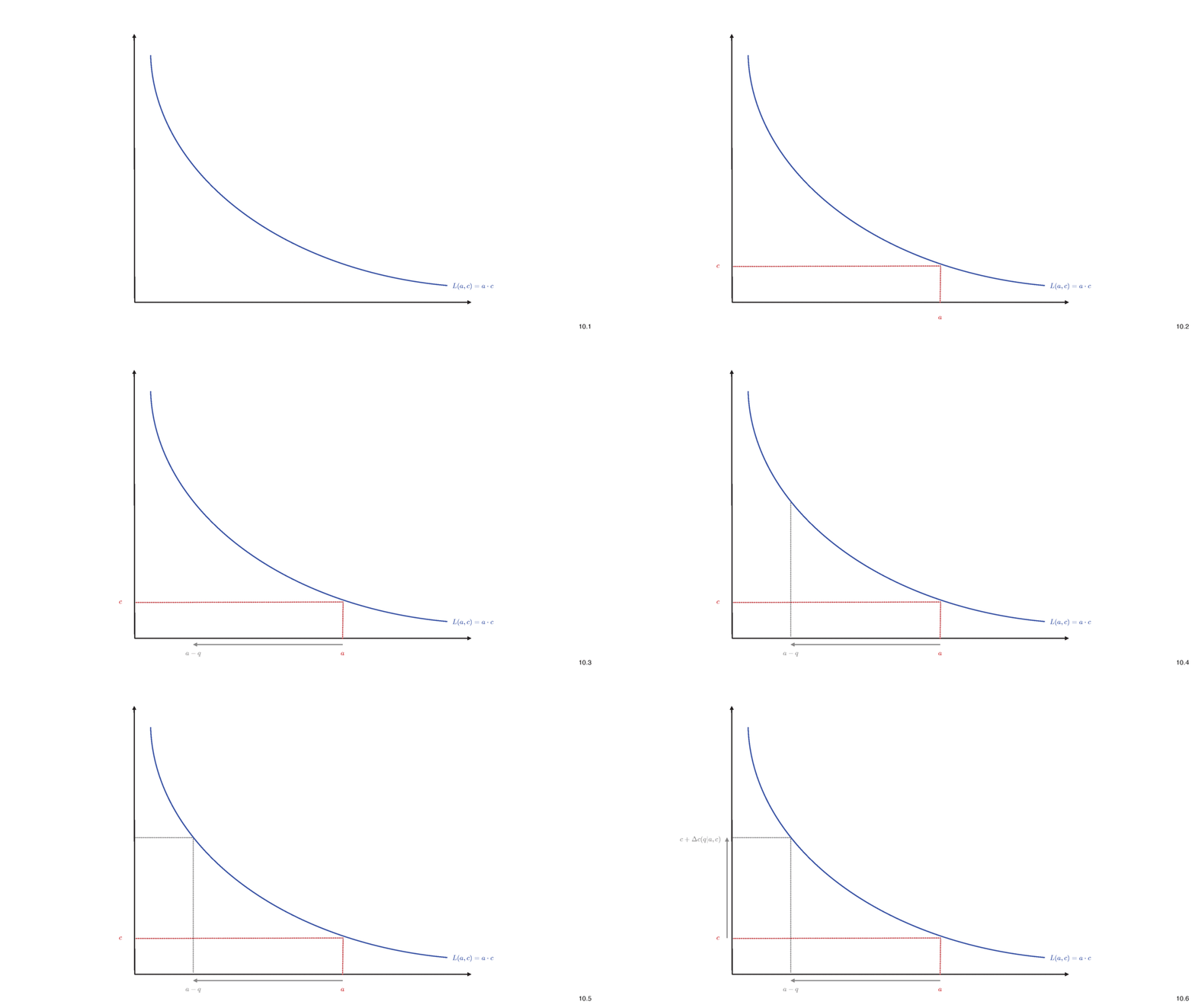
Constant Liquidity (Product) AMM
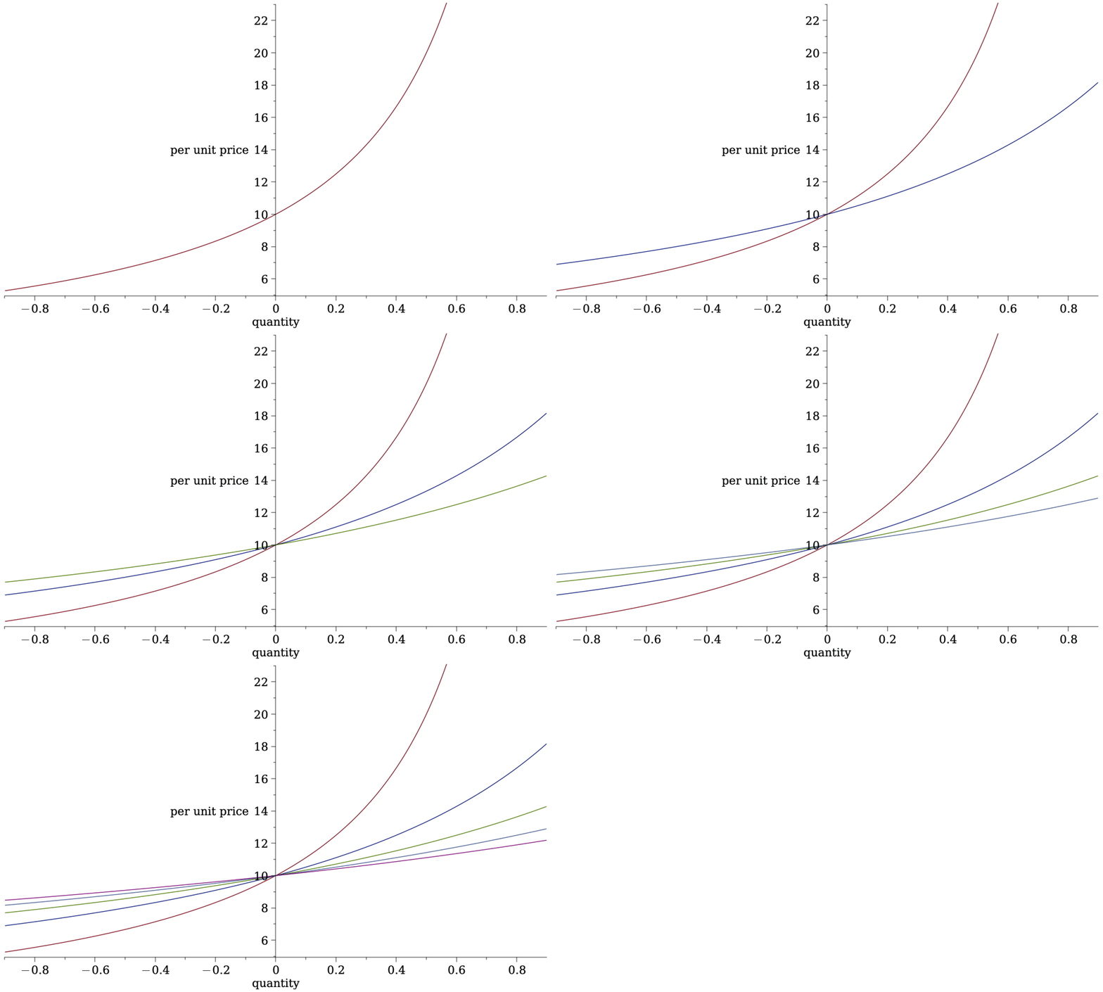
The Pricing Function
Basics of Liquidity Provision in an AMM for a Model
Basics of Liquidity Provision
\[E[\text{positional loss}(R)]+F\cdot E[\text{another function of }R]+F\cdot \frac{\text{dollar volume}}{\text{initial deposit}}\ge 0.\]
\[\text{LP payoff}=\text{what I sold it for}-\text{value of net position}+\text{fee income} \ge 0 \]
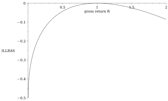
Sidebar: we can quantify how much a PASSIVE LP loses when the price moves by \(R\)
for orientation:
\[\frac{\text{adverse selection loss when the return is \(R\)}}{\text{initial deposit}}=\sqrt{R}-\frac{1}{2}(R+1)\equiv \textit{ILLRAS}(R)\]
as in Barbon & Ranaldo (2022)
"Incremental Loss from Long-Run Adverse Selection"
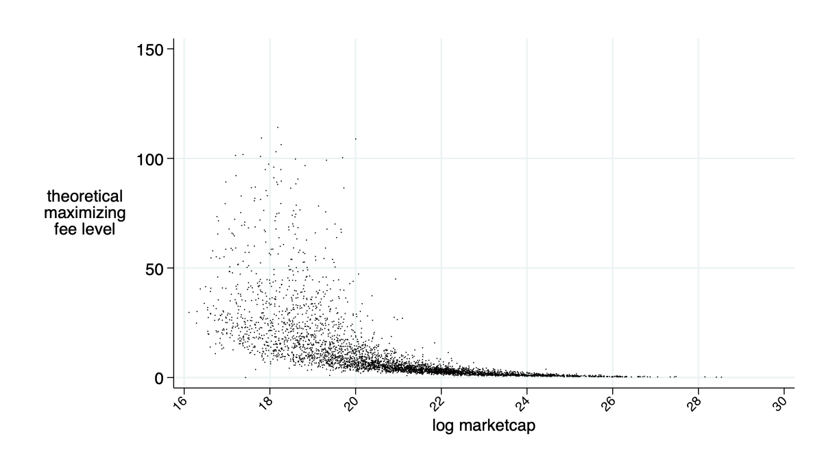
\[F^\pi=\frac{1}{E[|\sqrt{R}-1|/2]+V}\left(-2q\ E[\text{ILLRAS}]+ \sqrt{-2qV\ E[\text{ILLRAS}]}\right).\]
Liquidity Demander's Decision & (optimal) AMM Fees
Model Summary
How we think of the Implementation of an AMM for our Empirical Analysis
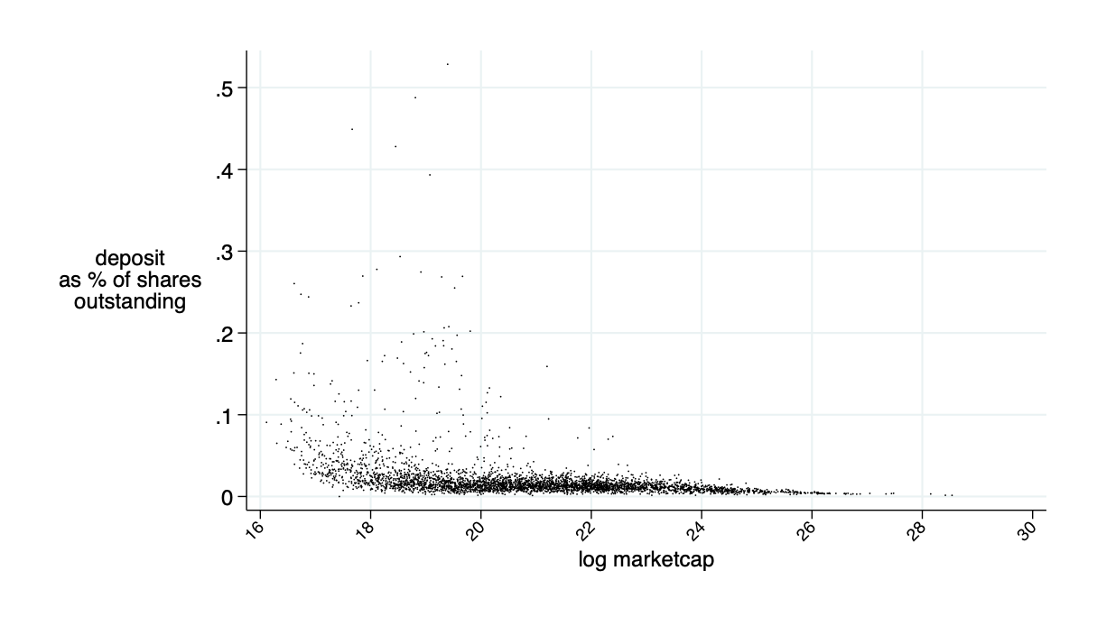
Approach: daily AMM deposits
Background on Data
some volume may be intermediated
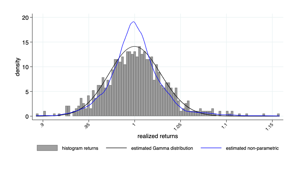
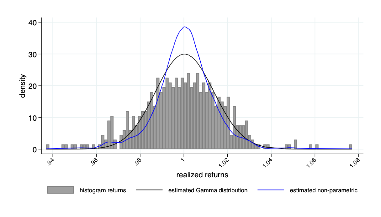
AMMs based on historical returns
Return distribution example: Microsoft
Return distribution example: Tesla
\(\bar{\alpha}\approx 2\%\)
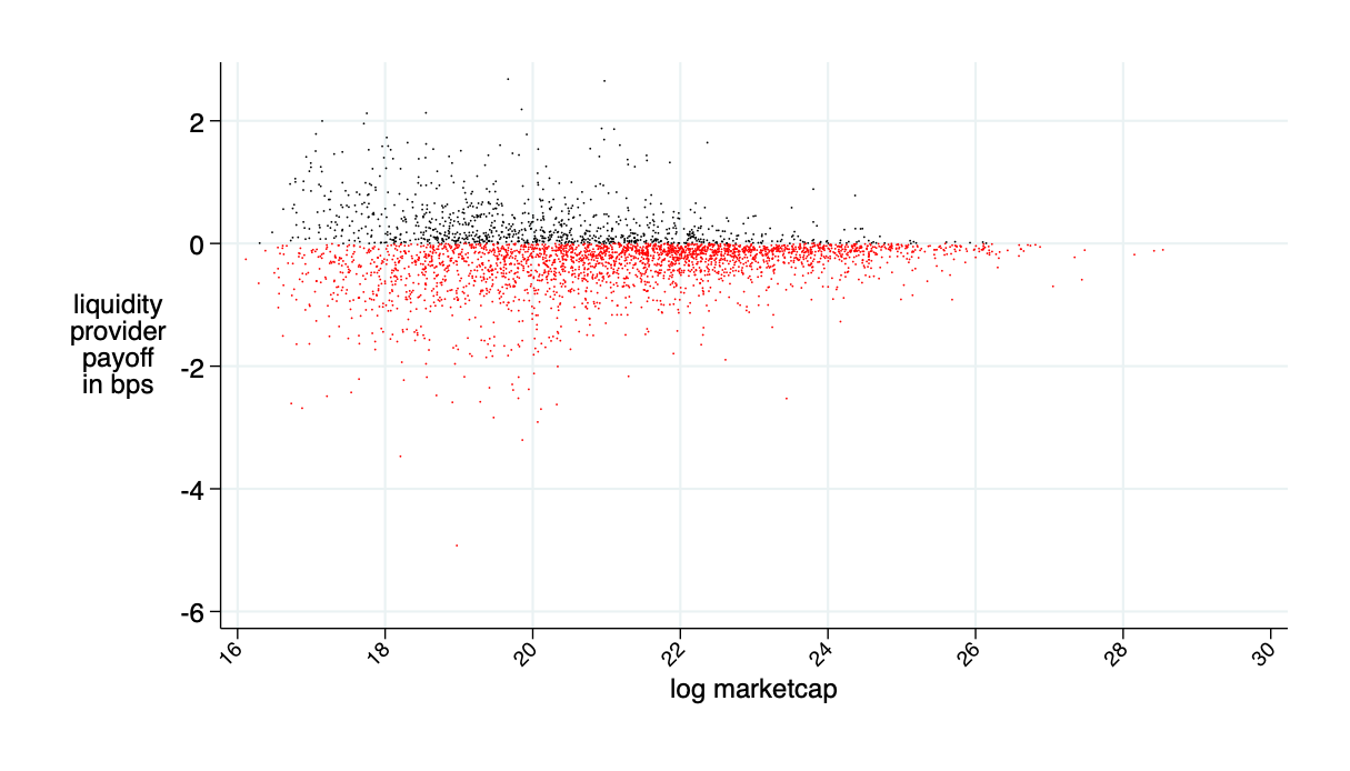
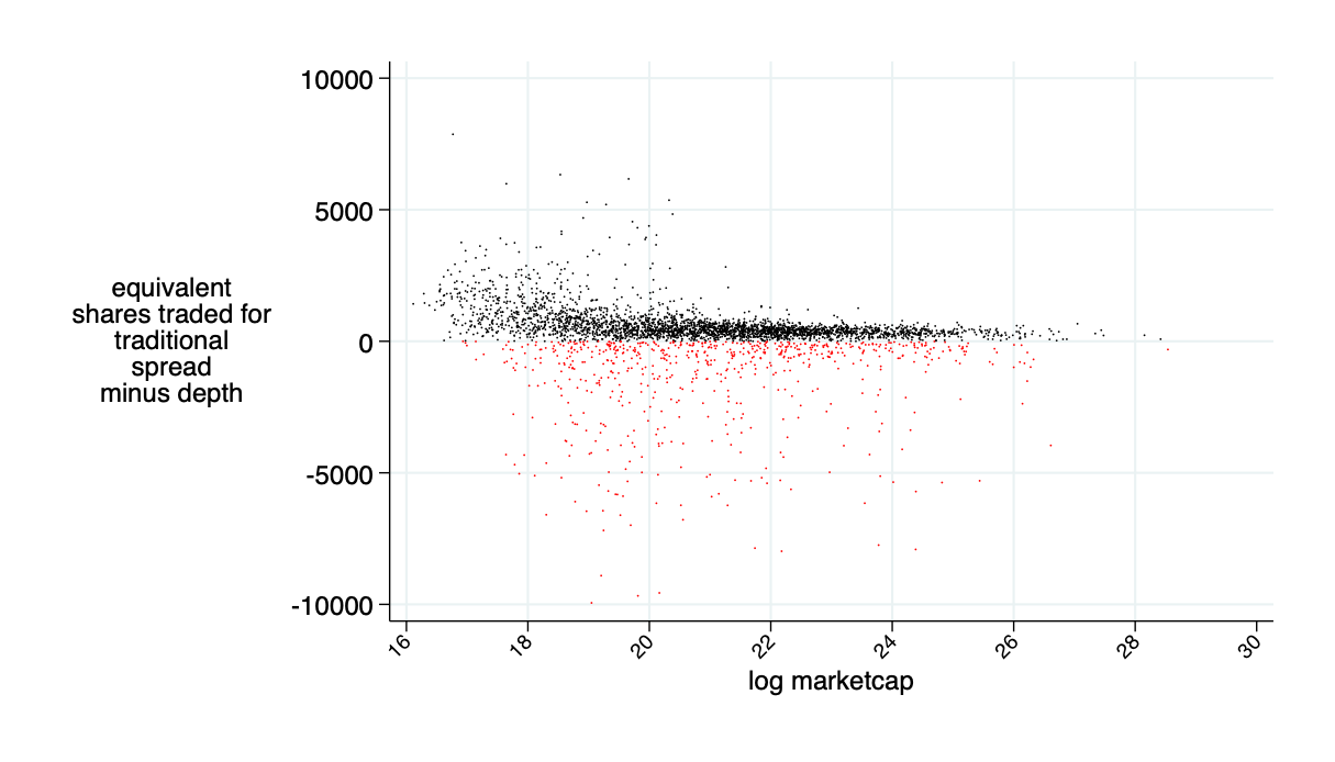
almost break even on average (average loss 0.2bps \(\approx0\))
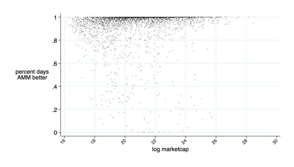
average: 94% of days AMM is better than LOB
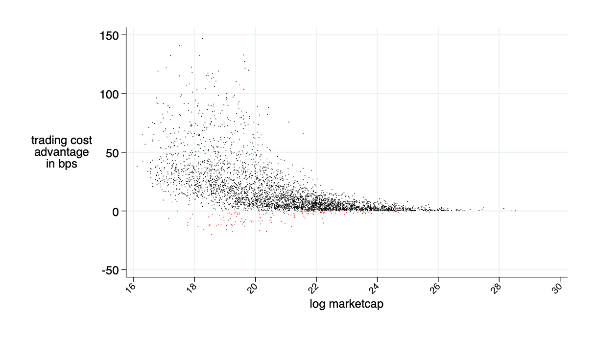
average savings: 16 bps
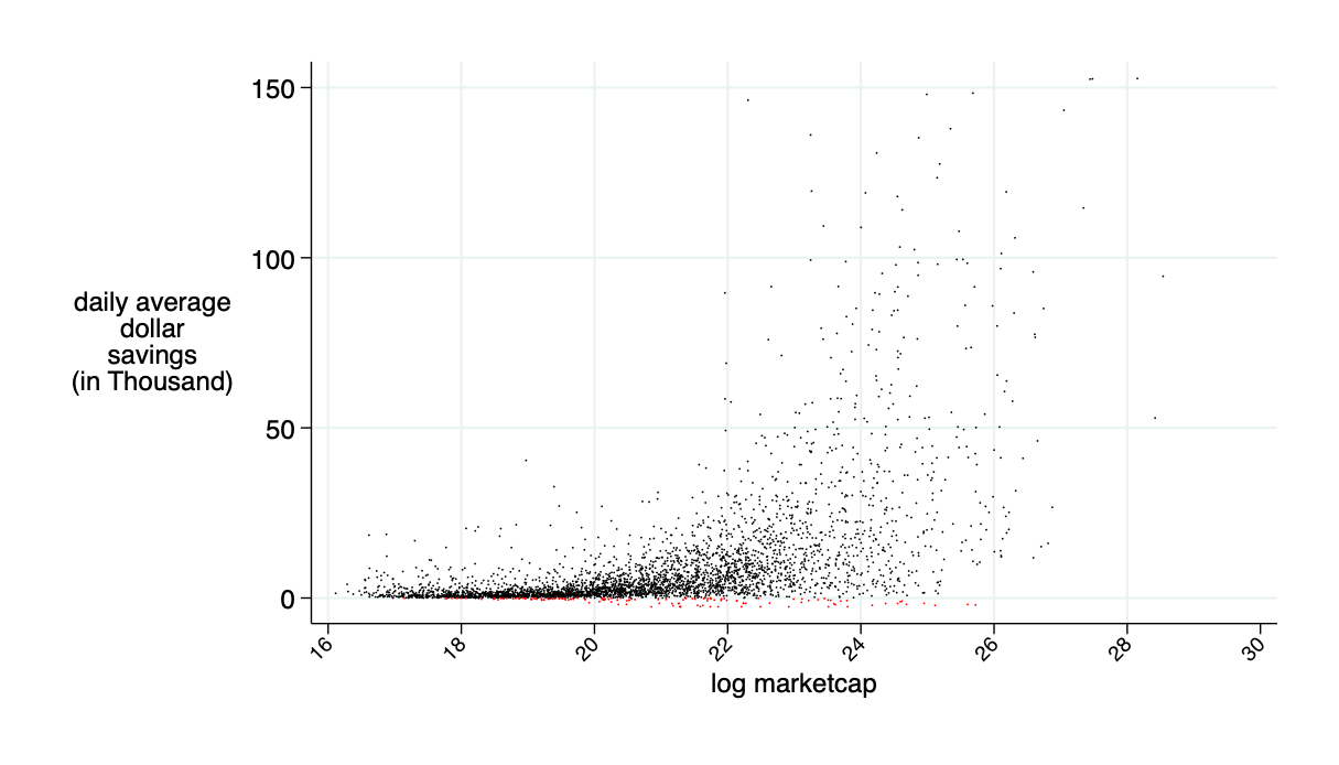
average daily: $9.5K
saves around 45% of transaction costs (measured in bid-ask spread)
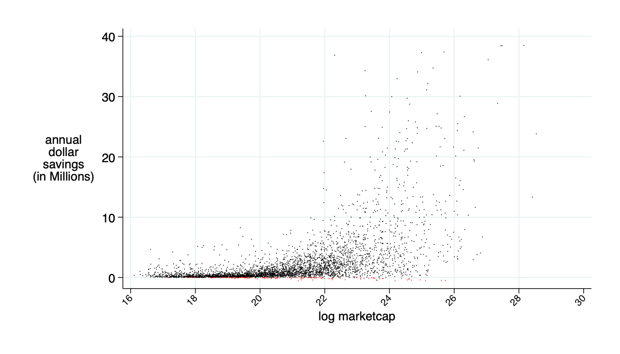
average annual saving: $2.4 million
Summary
@financeUTM
andreas.park@rotman.utoronto.ca
slides.com/ap248
sites.google.com/site/parkandreas/
youtube.com/user/andreaspark2812/
By Andreas Park
FedNY presentation