Stochastic Computation Graphs

Artëm Sobolev, AI Engineer at Luka Inc

@art_sobolev | http://artem.sobolev.name/

Outline of the talk

  • Intro
    • What (Stochastic) Computation Graphs are
    • Why study them
  • General Case
    • REINFORCE aka Score-Function Estimator
  • Continuous Case
    • Backprop through stochastic nodes
    • Reparameterisation Trick
    • Generalised Reparametrisation
  • Discrete Relaxations
    • Asymptotic Relaxation
    • Gumbel-Softmax
  • Fixing General Case
    • NVIL, MuProp, REBAR, Learnable baselines

Computational Graphs

  • Modern Deep Learning is all about differentiable computation graphs (directed and acyclic)
  • You can combine different layers as long as you can backpropagate through them
f(x|\phi) = f_1(f_2(... f_N(x|\phi_N) ... |\phi_2)|\phi_1)
f(xϕ)=f1(f2(...fN(xϕN)...ϕ2)ϕ1)f(x|\phi) = f_1(f_2(... f_N(x|\phi_N) ... |\phi_2)|\phi_1)
L(f(x|\phi), y) \to \min_\phi
L(f(xϕ),y)minϕL(f(x|\phi), y) \to \min_\phi
\nabla_\phi L(f(x|\phi), y)
ϕL(f(xϕ),y)\nabla_\phi L(f(x|\phi), y)

Stochastic Computational Graphs

  • Add stochastic layers \(z \sim p(z)\)
  • The task then becomes $$ \mathbb{E}_{p(z)} L(f(x, z|\phi), y) \to \min_\phi$$
  • Monte Carlo estimate the gradient if don't want to learn \(z\)'s parameters $$ \nabla_\phi L(f(x, z|\phi), y), z \sim p(z) $$

This talk: What if \(z \sim p(z|\theta)\)?

(and we'd like to find optimal \(\theta\) as well)

Stochastic Computational Graphs

  • General idea: we just need to figure out how to backpropagate through stochasticity
  • Our task is $$\mathbb{E}_{p(z|\theta)} F_\theta(z) \to \min_\theta$$
  • Let \(\mathcal{F}(\theta, \phi) = \mathbb{E}_{p(z|\theta)} F_\phi(z)\), then $$ \nabla_\theta \mathcal{F}(\theta, \theta) = \nabla_\theta F(\theta, \phi) \Bigr|_{\phi=\theta} + \nabla_\phi \mathcal{F}(\theta, \phi)\Bigr|_{\phi=\theta} $$
  • Backpropagation through \(F_\theta(z)\) is an easy problem, just backprop as usual with noise fixed
  • How to differentiate w.r.t. expectation's parameters?
  • See "Gradient Estimation Using Stochastic Computation Graphs" by J. Schulman et al.

Applications

General Case

REINFORCE

Let \(F(z) = L(f(x, z|\phi), y)\), then

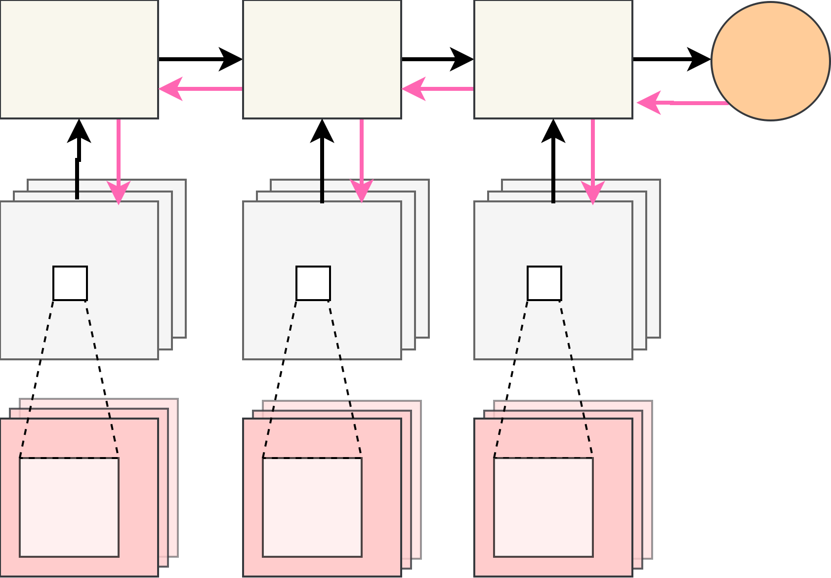
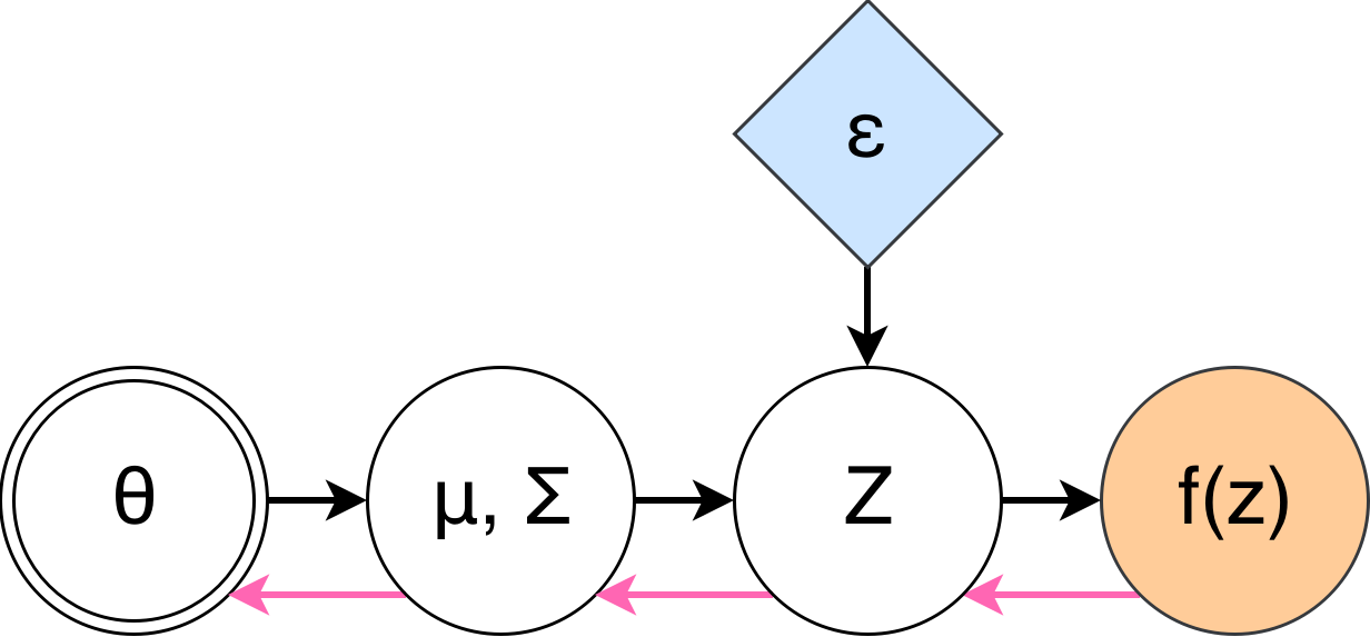
$$ \nabla_\theta \mathbb{E}_{p(z|\theta)} F(z) = \nabla_\theta \int F(z) p(z|\theta) dz = \int F(z) \nabla_\theta p(z|\theta) dz $$ $$= \int F(z) \nabla_\theta \log p(z|\theta) p(z|\theta) dz = \mathbb{E}_{p(z|\theta)} \nabla_\theta \log p(z|\theta) F(z) $$


Intuition: push probabilities of good samples (as measured by \(F(z)\)) up.

Pros: very general, does not require differentiable \(F\).

Cons: known to have large variance, sensitive to values of \(F\).


We'll get back to this estimator later in the talk.

Continuous Case

Backprop through sample

  • Can actually differentiate a sample w.r.t. its parameters!
  • For a univariate r.v. \(X_\theta\) with CDF \(\mathbb{F}(x|\theta)\) we have $$ \mathbb{F}(X_\theta|\theta) \sim U[0, 1] $$
  • Hence $$ 0 = \frac{\partial}{\partial \theta} \mathbb{F}(X_\theta |\theta) = \frac{\partial}{\partial \theta} \mathbb{F}(x|\theta)|_{x=X_\theta} + p(X_\theta) \frac{\partial}{\partial \theta} X_\theta $$ $$ \frac{\partial X_\theta}{\partial \theta} = - \frac{1}{p(X_\theta)} \int_{-\infty}^{X_\theta} \frac{\partial}{\partial \theta} p(x|\theta) dx$$
  • Extends to multivariate case with conditional marginal CDFs


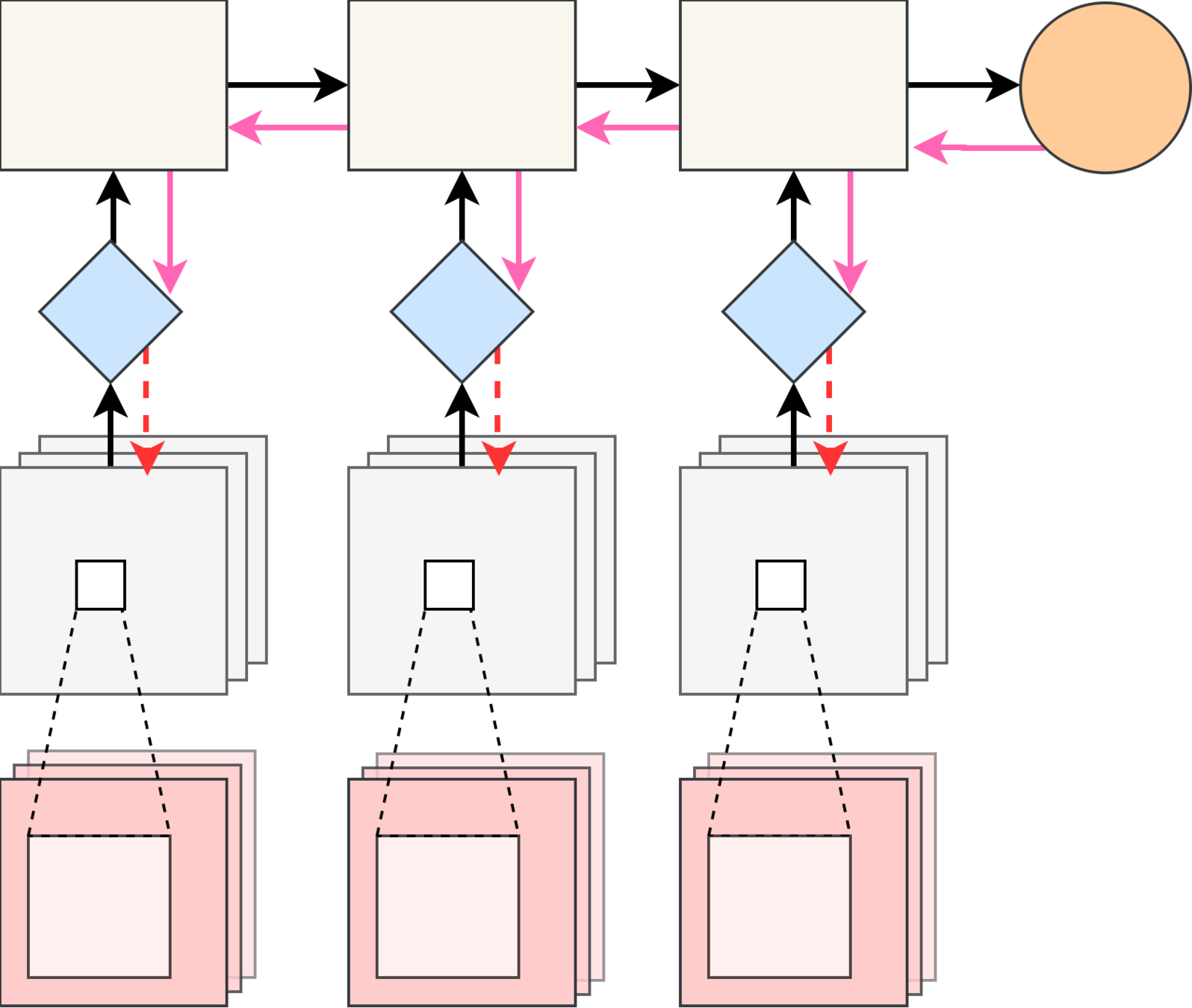
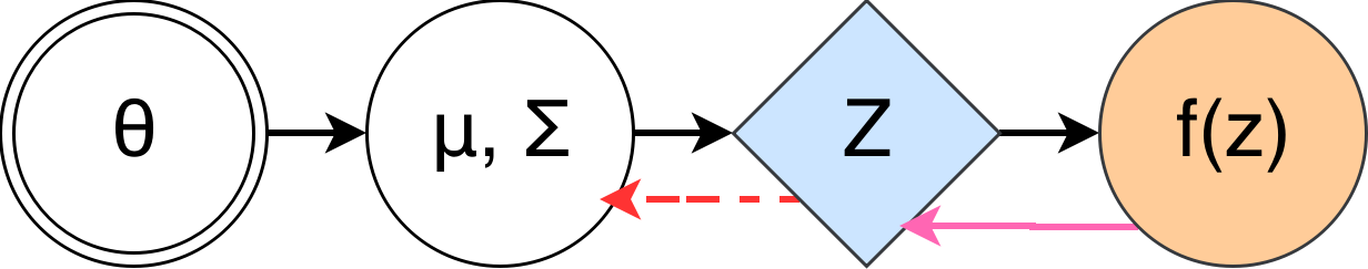
Pros: backprop through sample

Cons: requires ability to differentiate CDF w.r.t. \(\theta\)

Reparametrisation Trick

  • Stochastic Computation Graph with Gaussian hidden nodes: $$ z|x \sim \mathcal{N}(z \mid \mu(x|\theta), \Sigma(x|\theta)) $$
  • \(z|x\) has the same distribution as \(\mu(x|\theta) + \Sigma(x|\theta)^{1/2} \varepsilon \)

ReparametriSation Trick

  • If \(z|\theta\) has the same distribution as \(\mathcal{T}_\theta(\varepsilon) \) for some differentiable \(\mathcal{T}_\theta\)
  • Then $$ \mathbb{E}_{p(z|\theta)} F(z) = \mathbb{E}_{p(\varepsilon)} F(\mathcal{T}_\theta(\varepsilon)) $$ $$ \nabla_\theta \mathbb{E}_{p(z|\theta)} F(z) = \mathbb{E}_{p(\varepsilon)} \nabla_\theta F(\mathcal{T}_\theta(\varepsilon)) $$


  • Pros: obtained estimator is very efficient in practise
  • Cons:
    • not every distribution has a useful reparametrisation (e.g. Dirichlet distribution)
    • requires differentiable \(F\)

GeneraliSed ReparametriSation Trick

  • Idea: reparametrisation removes dependence on parameters completely. What if we remove it just partially?
  • For example, whiten first moments: $$ \varepsilon = \mathcal{T}_\theta^{-1}(z) = \frac{z - \mu(\theta)}{\sigma(\theta)} \quad\quad z = \mathcal{T}_\theta(\varepsilon) $$
  • \(\varepsilon\) still depends on \(\theta\): \(\varepsilon \sim p(\varepsilon|\theta)\)

$$ \nabla_\theta \mathbb{E}_{p(\varepsilon|\theta)} F(z) = \mathbb{E}_{p(\varepsilon|\theta)} \nabla_\theta F(\mathcal{T}_\theta(\varepsilon)) + \mathbb{E}_{p(\varepsilon|\theta)} \nabla_\theta \log p(\varepsilon|\theta) F(\mathcal{T}_\theta(\varepsilon))$$

  • The first term is reparametrised gradient, the second is the correction to make the gradient unbiased.
  • Can also be seen from the rejection sampling perspective *
    • Don't need the \(\mathcal{T}^{-1}_\theta\) then

GeneraliSed ReparametriSation Trick

The formula $$ \nabla_\theta \mathbb{E}_{p(\varepsilon|\theta)} F(z) = \mathbb{E}_{p(\varepsilon|\theta)} \nabla_\theta F(\mathcal{T}_\theta(\varepsilon)) + \mathbb{E}_{p(\varepsilon|\theta)} \nabla_\theta \log p(\varepsilon|\theta) F(\mathcal{T}_\theta(\varepsilon))$$ requires us to sample \( \varepsilon|\theta\). With a bit of algebra we can rewrite these addends in terms of samples \(z|\theta\): $$ \mathbb{E}_{p(z|\theta)} \nabla_z F(z) \nabla_\theta h_\theta(\mathcal{T}^{-1}_\theta(z)) $$ $$\mathbb{E}_{p(z|\theta)} F(z) \left[ \nabla_\theta \log p(z|\theta) + \nabla_z\log p(z|\theta) h_\theta(\mathcal{T}^{-1}_\theta(z)) + u_\theta(\mathcal{T}^{-1}_\theta(z))\right]$$

Where

  • \(h_\theta(\varepsilon) = \nabla_\theta \mathcal{T}_\theta(\varepsilon)\) – Jacobian of \(\mathcal{T}_\theta\) w.r.t. \(\theta\)
  • \(u_\theta(\varepsilon) = \nabla_\theta \log \Bigl|\text{det} \nabla_\varepsilon \mathcal{T}_\theta(\varepsilon)\Bigr| \)

Pros: interpolates between reparametrisation and REINFORCE

Cons: need to come up with differentiable \(\mathcal{T}_\theta\)

Simple Example

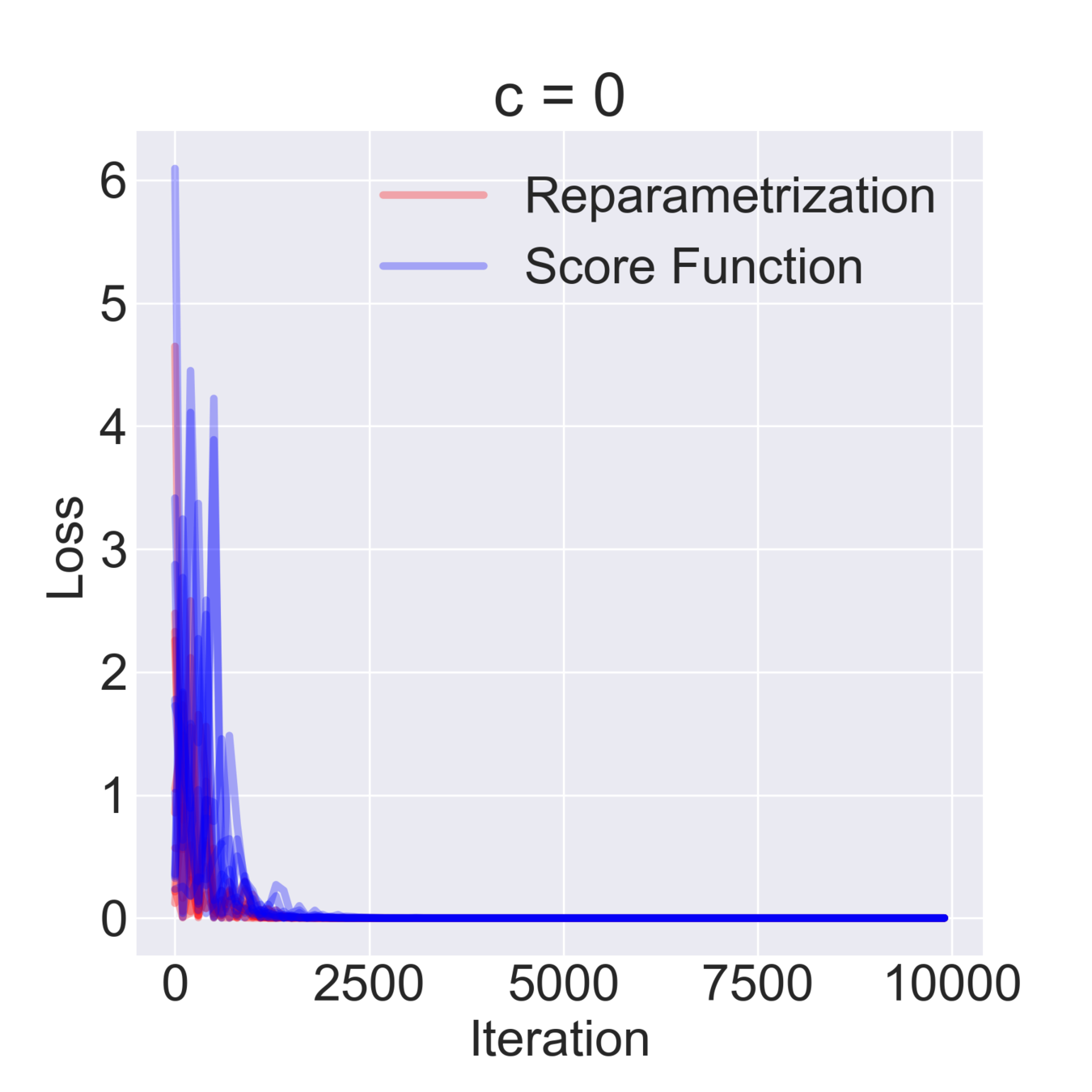
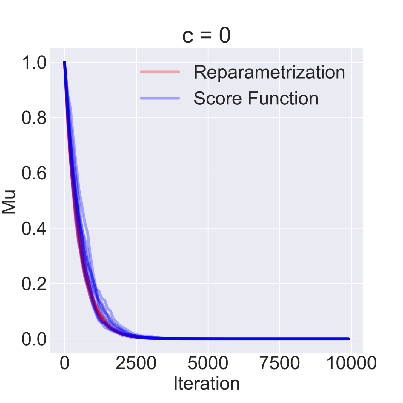
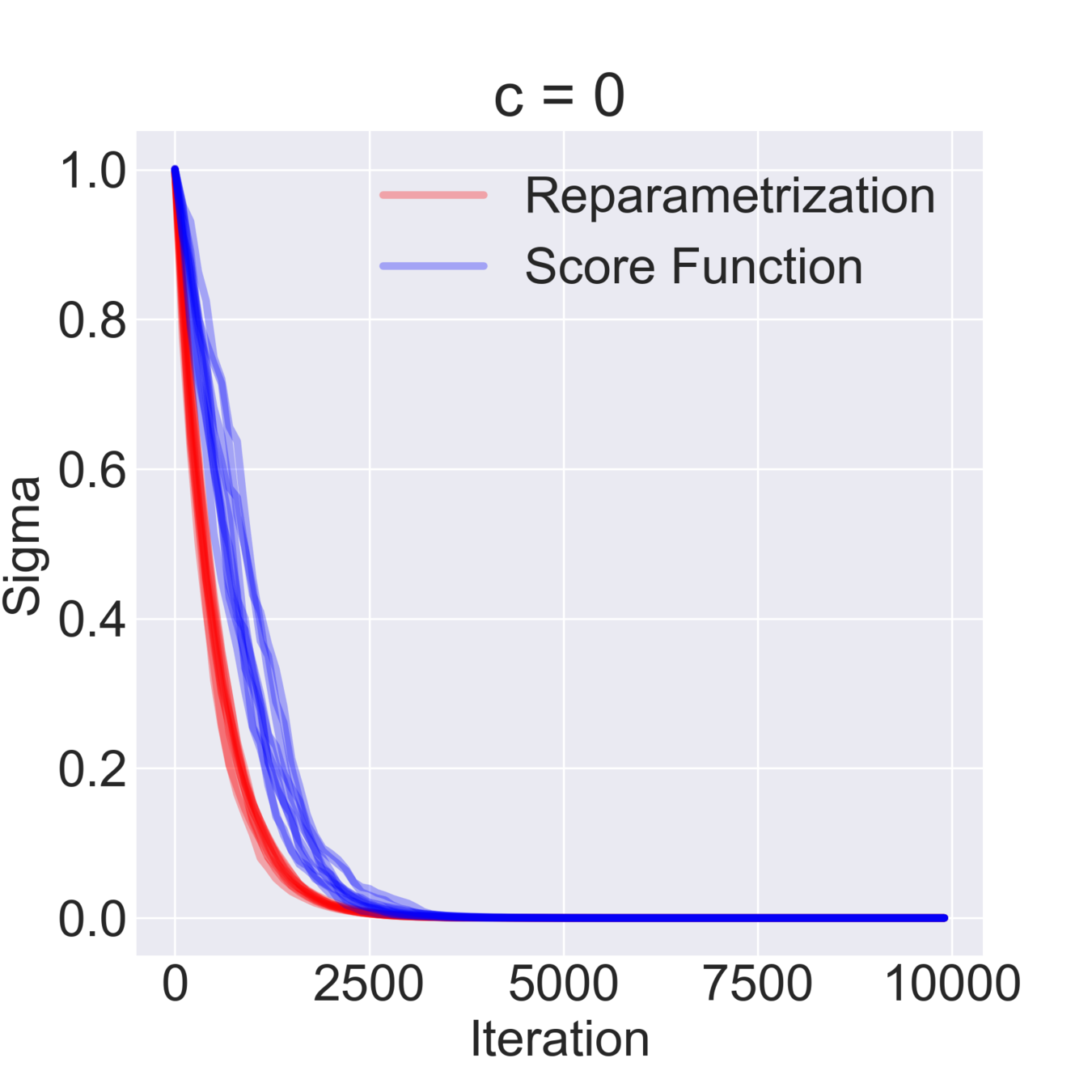
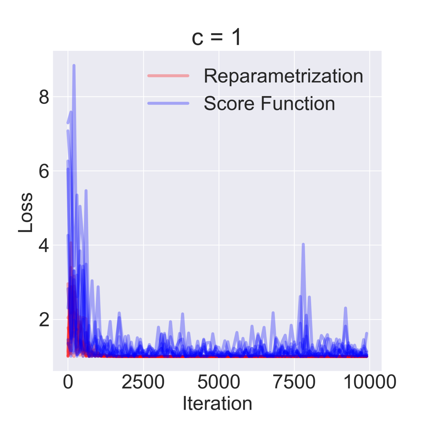
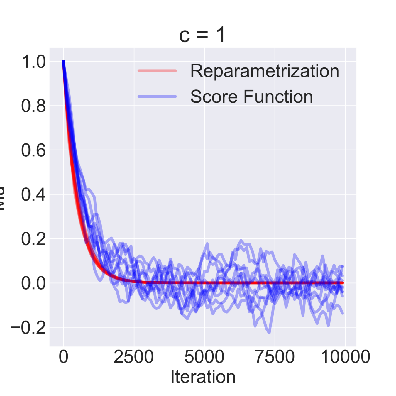
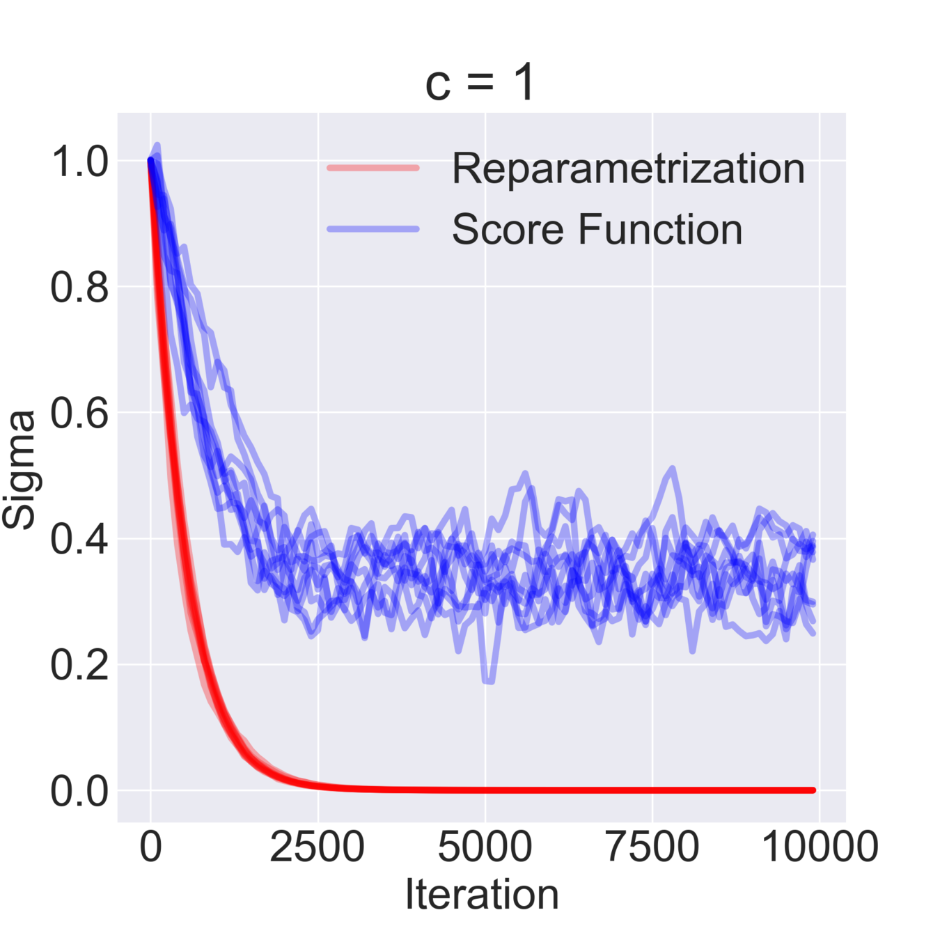
$$ \mathcal{F}(\mu, \sigma) = \mathbb{E}_{z \sim \mathcal{N}(\mu, \sigma^2)} [z^2 + c] = \mathbb{E}_{\varepsilon\sim\mathcal{N}(0, 1)} [(\mu + \varepsilon \sigma)^2 + c] \to \min_{\mu, \sigma} $$

$$ \hat \nabla_\mu \mathcal{F}^{\text{rep}}(\mu, \sigma) = 2 (\mu + \sigma \varepsilon) \quad\quad \hat\nabla_\mu \mathcal{F}^\text{SF}(\mu, \sigma) = \frac{\varepsilon}{\sigma} ((\mu+\sigma \varepsilon)^2+c) $$

$$ \hat \nabla_\sigma \mathcal{F}^\text{rep}(\mu, \sigma) = 2 \varepsilon (\mu + \sigma \varepsilon) \quad\quad \hat \nabla_\sigma \mathcal{F}^\text{SF}(\mu, \sigma) = \frac{\varepsilon^2-1}{\sigma}((\mu+\sigma \varepsilon)^2+c)$$

$$ \mathbb{D}[\hat \nabla_\mu \mathcal{F}^\text{rep}(\mu, \sigma)] = 4 \sigma^2 \quad\quad \mathbb{D} [\hat \nabla_\sigma \mathcal{F}^\text{rep}(\mu, \sigma)] = 4 \mu^2 + 8 \sigma^2 $$

$$ \mathbb{D}[\hat \nabla_\mu \mathcal{F}^\text{SF}(\mu, \sigma)] = \frac{(\mu^2 + c)^2}{\sigma^2} + 15 \sigma^2 + 14 \mu^2 + 6 c $$

$$ \mathbb{D}[\hat \nabla_\sigma \mathcal{F}^\text{SF}(\mu, \sigma)] = \frac{2 (\mu^2 + c)^2}{\sigma^2} + 74 \sigma^2 + 60 \mu^2 + 20 c $$

Simple Example

Simple Example

Simple Example

Simple Example

Simple Example

Mu

Simple Example

Discrete relaxations

AsympToTic reparametrisation

  • Suppose you have binary dropout and want to adjust each neuron's dropout rate.
  • Consider a pair of layers \(h_1\) and \(h_2\) such that \( h_2 = \sigma(W h_1 + b) \)
  • Dropout:  \( h_2 = \sigma(W (h_1 \circ z) + b), \quad z \sim \text{Bernoulli}(p) \)
  • Dropout masks only enter sums with many addends
  • We might hope for CLT to hold
  • Hopefully preactivations of \(h_2\) are approximately normal:
    • Mean \( W(h_1 \circ \mathbb{E} z) + b = W (h_1 \circ p) + b\)
    • Covariance \( W \mathbb{D} z W^T = W (p \circ (1-p)) W^T\)
  • Equivalent to multiplicative \(\mathcal{N}(p, p(1-p))\) noise


  • Pros: benefits of Gaussian Reparametrisation
  • Cons: very limited applicability scope, depends on how good the CLT approximation is

Gumbel-Softmax Relaxation

  • Can use any continuous r.v. \(X\) with CDF \(\mathbb{F}(x)\) to generate \(\text{Bernoulli}(p)\) r.v. by $$ z = [X> \mathbb{F}^{-1}(1-p)] = H(X- \mathbb{F}^{-1}(1-p))$$
  • Approximate the step function using a sigmoid function with temperature: $$ H(x-a) = \lim_{\tau \to 0} \sigma(\tfrac{x-a}{\tau}) $$


  • Which \(X\) to choose?
    • Sample values close to 0 and 1 more often
      • ⇒ need modes there
      • ⇒ \(X\) should have all \(\mathbb{R}\) as a support
    • Want to be able to relax general categorical r.v.


  • Gumbel-Max Trick will help

Gumbel-Max To Gumbel-Softmax

  • Gumbel random variables \(\{\gamma_k\}_{k=1}^K\) have a nice property: $$ \mathbb{P}(k = \text{argmax}_j [\gamma_j + \log p_j]) = \frac{p_k}{\sum_j p_j} $$
  • Gumbel-Max Trick: Sample categorical r.v. via maximisation of independently perturbed log-probabilities


  • Suppose argmax returns a one-hot vector
  • Approximate it with a softmax with temperature $$ \text{argmax}(x) = \lim_{\tau \to 0} \text{softmax}(\tfrac{x}{\tau}) $$ (temperature makes outputs more contrast)

$$ z = \text{argmax}_k \left[\gamma_k + \log p_k\right] $$

$$ \zeta = \text{softmax}_\tau \left(\gamma_k + \log p_k\right) $$

Pros: works in categorical case, temperature controls bias

Cons: still biased, not clear how to tune temperature

Gradient relaxation

Many other estimators only relax the backward pass

  • Straight Through Estimator: backpropagate through hard thresholding as if it was an identity function: $$\tfrac{\partial}{\partial \theta} H(x - \sigma(-\theta)) = 1$$
  • Or one might keep the derivative of \(\sigma\): $$H'(x) = 1 \Rightarrow \tfrac{\partial}{\partial \theta} H(x - \sigma(-\theta)) = \sigma(\theta) \sigma(-\theta)$$
  • Gumbel Straight Through: backward pass as in the Gumbel-Softmax relaxation


Pros: don't see any

Cons: mathematically unsound ¯\_(ツ)_/¯

Example: Discrete Variational Autoencoder

  • Modeling discrete data using discrete latent representation
  • Bernoulli model: $$z \sim \text{Bernoulli}(p), \quad\quad x|z \sim \text{Bernoulli}(\mu(z))$$
  • Amortised Variational Inference: $$ q(z|x) = \prod_{k=1}^K \text{Bernoulli}(z_k|\kappa(x)_k) $$
  • Objective: $$ \mathcal{L}(\mu, \kappa) = \mathbb{E}_{q(z|x)} \log \frac{p(x, z)}{q(z|x)} = \mathbb{E}_{q(z|x)} \log p(x|z) - D_{KL}(q(z|x)||p(z))$$ We will compute the second term analytically, and relax the first one
  • Evaluation: multi-sample lower bound for L=10,000 samples: $$\mathcal{L}_k(\mu, \kappa) = \mathbb{E}_{q(z|x)} \log \frac{1}{L} \sum_{l=1}^L \frac{p(x, z_l)}{q(z_l|x)} $$ in the limit approaches marginal log-likelihood \(\log p(x)\)

Discrete Variational Autoencoder

Discrete Variational Autoencoder

Discrete Variational Autoencoder

Fixing REINFORCE

Back to REINFORCE

  • REINFORCE gradient estimate: \( \nabla_\theta \log p(z|\theta) F(z) \)
  • We've seen how offsetting \(F(z)\) can break the estimator


  • Easy to fix by just centring \(F(z)\)
  • Leads to a baseline: \( b \nabla_\theta \log p(z|\theta) \)
  • Optimal \(b\) can be found analytically, and estimated using moving averages


  • Pros: Simple, sparse gradients
  • Cons: Not efficient enough

What do we even want?

  • We've seen some methods and experiments, time to ask ourselves "What could make REINFORCE more efficient?"
  • Control Variates: $$ \mathbb{E}_{p(z|\theta)} \left[F(z) \nabla_\theta \log p(z|\theta) + B(z)\right]- \mathbb{E}_{p(z|\theta)} B(z)$$ if \(B(z)\) and \(F(z) \nabla_\theta \log p(z|\theta)\) are negatively correlated, resulting estimator has lower variance.

How to design a control variate?

  • Using prior information (dependency structure) often helps
  • Gradient information \(\nabla_z F(z)\) should help
  • Good baselines "integrate out" as much as possible:
    • Ideally we'd like to decompose REINFORCE estimate into easy to work with parts
    • Or at least reduce its influence
    • Thus likely to use samples \(z\)

NVIL estimator

  • Neural Variational Inference and Learning in Belief Networks
  • Very similar to what RL people do
  1. Centring learning signal: $$ \mathbb{E}_{p(z|x, \theta)} [F(x, z) - \color{red}{b(x) - C}] \nabla_\theta \log p(z|x, \theta)$$ (\(b(x)\) does not have to be scalar)
  2. Variance Normalisation: divide by estimate of standard deviation.
  3. Local learning signals: exploit inner structure of \(p(z|x, \theta)\) and \(F(x,z)\)
    • Akin to using cumulative future reward in RL
  • VIMCO: extension to multi-sample objectives

Pros: more efficient, still easy to implement

Cons: requires training an extra model \(b(x)\) (unless VIMCO), does not use \(z\) in the baseline, doesn't use gradient \(\nabla_z F(z)\)

MuProp estimator

  • Idea: use first-order Taylor approximation as a baseline $$ F(z) \approx F(\zeta) + \nabla F(\zeta)^T (z - \zeta) $$
  • Easy to fix the bias: $$ \mathbb{E}_{p(z|\theta)} \nabla F(\zeta)^T z \nabla_\theta \log p(z|\theta) = \nabla_\theta \mathbb{E}_{p(z|\theta)} \nabla F(\zeta)^T z = \nabla F(\zeta)^T \nabla_\theta \mathbb{E}_{p(z|\theta)} z $$
  • \(\zeta\) is chosen as a "mean-field" point


Pros: uses gradient information \(\nabla_z F(z)\)

Cons:

  • Need to compute \(\mathbb{E}_{p(z|\theta)} z\) analytically to backprop through it
  • Only a first order approximation

REBAR estimator

  • Idea: use Gumbel-Softmax relaxation as a baseline
  • Turns out can compensate for the bias


  • Assume \( z|\theta = H(X|\theta)\), then $$ \mathbb{E}_{p(X|\theta)} F(z) \nabla_\theta \log p(z|\theta) = \mathbb{E}_{p(X|\theta)}F(H(X|\theta)) \nabla_\theta \log p(X|\theta)$$ RHS has high variance due to non-marginalised sampling
  • Control variate: $$ \mathbb{E}_{p(X|\theta)} F(\sigma_\tau(X)) \nabla_\theta \log p(X|\theta) = \nabla_\theta \mathbb{E}_{p(X|\theta)} F(\sigma_\tau(X))$$
  • Can conditionally marginalise the estimator

\( \nabla_\theta \mathbb{E}_{p(X|\theta)} F(\sigma_\tau(X)) = \nabla_\theta \mathbb{E}_{p(X, z|\theta)} F(\sigma_\tau(X)) = \)

$$ \mathbb{E}_{p(z|\theta)} \left[\nabla_\theta \mathbb{E}_{p(X|z, \theta)} F(\sigma_\tau(X|z))\right] + \mathbb{E}_{p(z|\theta)} \mathbb{E}_{p(X|z,\theta)} [F(\sigma_\tau(X|z))] \nabla_\theta \log p(z|\theta) $$ 

REBAR estimator

We arrive to the following formula

$$\nabla_\theta \mathbb{E}_{p(z|\theta)} F(z) = \mathbb{E}_{u, v} \left[ \left(F(z) - \eta F(\zeta|z) \right) \nabla_\theta \log p(z|\theta) + \eta \nabla_\theta F(\zeta) - \eta \nabla_\theta F(\zeta|z) \right]$$ 

Where \(z=H(X)\), \(\zeta = \sigma_\tau(X)\), \(\zeta|z = \sigma_\tau(X|z)\)

\( X = \log \frac{u}{1-u} + \log \tfrac{\mu(\theta)}{1-\mu(\theta)} \)

\(\eta\) and \(\tau\) are tuneable parameters, optimised to reduce the variance

Pros:

  • uses \(F\)'s gradient information
  • quality of approximation is controlled by temperature
  • essentially Gumbel-Softmax with bias removed

Cons:

  • quite involved
  • requires several evaluations of \(F\)

Extra: From REBAR to RELAX

What if \(F(z)\) is not differentiable or we don't know its gradients (like in RL)?

  • If \(z\) is continuous and reparametrisable, we can learn a baseline \(c(z)\): $$ \hat g = (F(z) - \tilde{F}(z)) \nabla_\theta \log p(z|\theta) + \nabla_\theta \tilde{F}(z), \quad z = \mathcal{T}(\varepsilon|\theta), \varepsilon \sim p(\varepsilon)$$We reparametrised the last term; \(\tilde{F}\) is optimised to minimise the variance of this gradient estimate
  • Discrete case: relax \(z\) just as in REBAR, gives us $$\hat g = (F(z) - \eta \tilde{F}(\zeta|z)) \nabla_\theta \log p(z|\theta) + \eta \nabla_\theta F(\zeta) - \eta \nabla_\theta F(\zeta|z) $$

The \(\tilde{F}\) is optimized to minimize the variance $$\text{Var} \hat{g}_i = \mathbb{E} \hat{g}_i^2 - \left(\mathbb{E} \hat{g}_i\right)^2$$ \(\hat{g}_i\) is unbiased, hence the second term does not depend on \(\tilde{F}\)

Conclusion

  • We reviewed many techniques to backpropagate through stochastic nodes 
  • Continuous Case has efficient unbiased gradient estimators
    • And yet it's possible to reduce the variance even further
  • Discrete Case is still an open problem:
    • Many different biased relaxations, not clear which to use
    • Variance Reduction techniques might still have large variance
  • Many other methods left uncovered
  • DVAEs can be found here (work in progress): https://github.com/artsobolev/dvaes

Stochastic Computation Graphs

By Artëm Sobolev

Stochastic Computation Graphs

My talk on stochastic computation graphs for BayesGroup seminar

  • 2,782