Stochastic Models of Early HIV Infection
Bernhard Konrad
Institute of Applied Mathematics
The University of British Columbia
March 30th, 2015
HIV/AIDS - a deadly pandemic
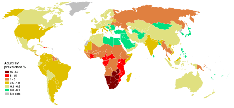
- 35M individuals living with HIV today
- 36M AIDS-caused deaths total (1.6M in 2012)
- 2.3M new HIV infections in 2012
HIV/AIDS close to home
Canada
- 70,000 HIV+ (2009)
- 2,500 new diagnosis every year
- one new infection every 3h
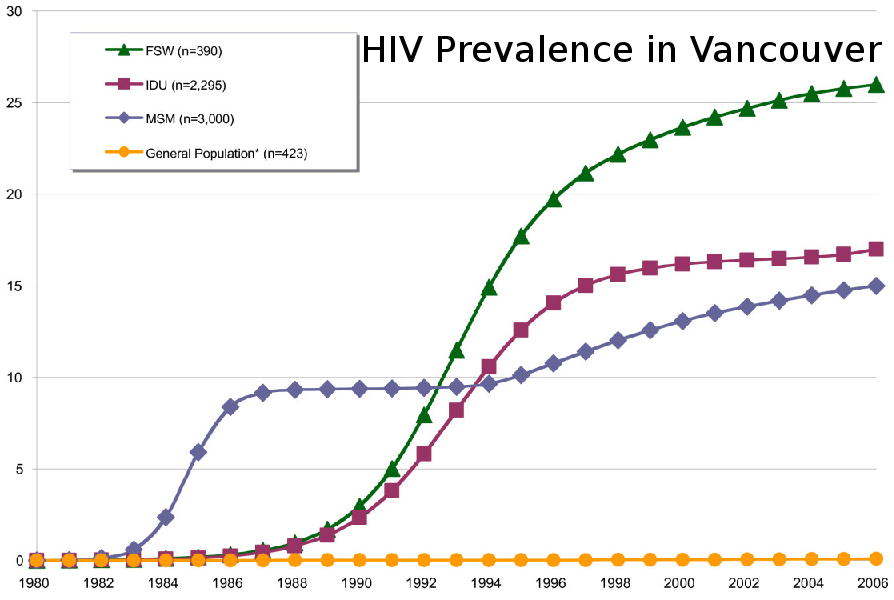
BC
- 400 new diagnosis every year
- 3,500 unaware of infection (25%)
Epidemiology with BCCDC

Survey Data from epidemiologists at the BCCDC in Vancouver:
- ManCount
- SexNow
- GetCheckedOnline
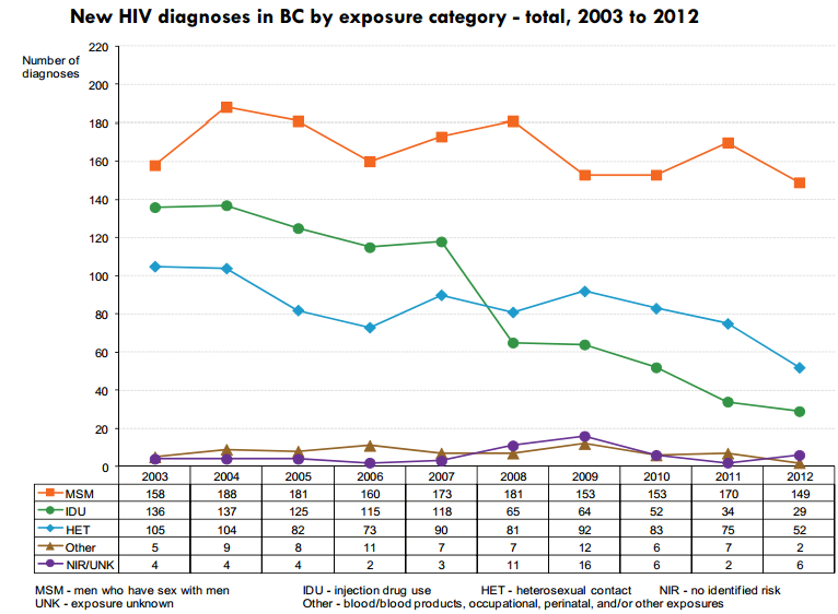
Data mining, visualization, and modelling to gain actionable insight and predict the outcome of health interventions in the Vancouver HIV MSM epidemic.
Immunology of HIV infection
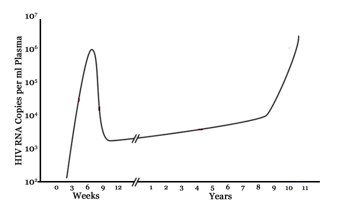
- several weeks for potent antibody response to mount
- symptoms at infection very mild or completely absent
Importance of Early Infection
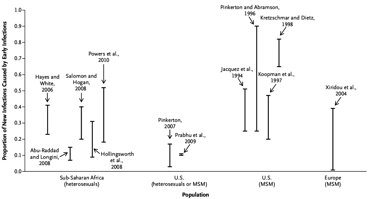
- Extremely high viral load
- Sexually active
- Unaware of infection
Importance of Early Infection
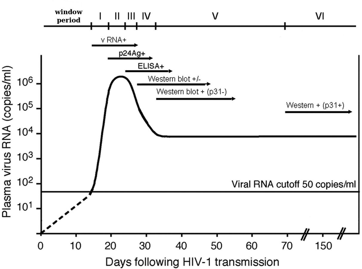
- Different HIV tests look for different signals...
- ...and become positive at different times
Importance of Early Infection
- Work so far has focused on calculating relative time delay between Fiebig Stages
Research Question
- How long is the window period?
- Given a negative HIV test t days after possible exposure, how likely is an infection?
- When to schedule second, confirmatory test?
Mathematical formulation
- Distribution of the length of the window period?
- What is the probability that the number of virions is large enough to be detectable by a HIV test at time t?
- What is the probability that a patient is infected, given a negative test result at time t?
Data
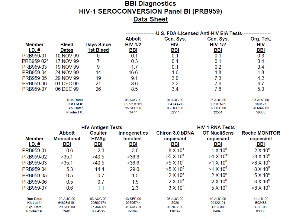
- Plasma samples from regular donors
- Stored before putting put in use
- Removed if any infection detected in a later sample
- Very valuable in research for benchmarking new tests
Data
Data
- Data collected (bought by BCCDC) from several sources
- Stored in several csv files
- Usually several tests for the same patient sample
- duplicates (easy)
- lower and upper detection limits
- different HIV tests (usually trust "better" test)
- correctly average if tests disagree
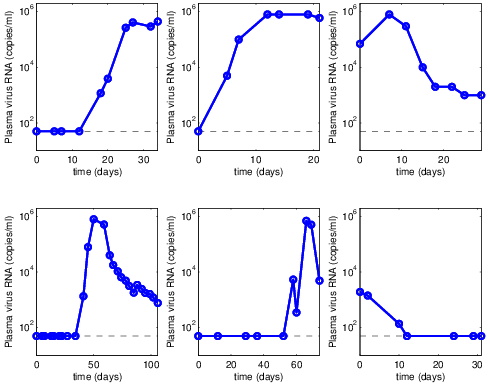
- Importance of visualization
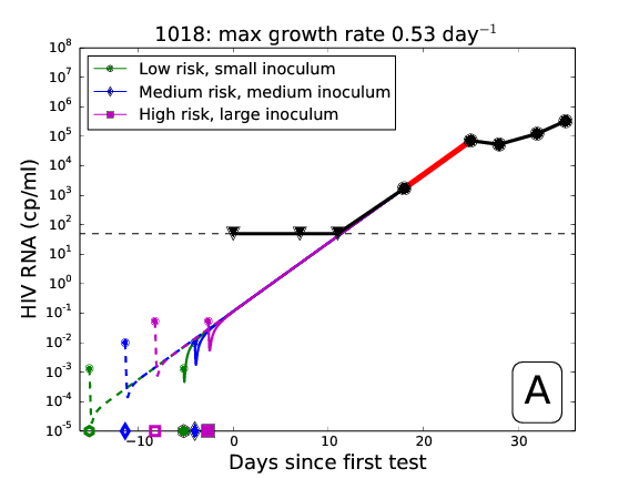
Mathematical Model
- Detection limit 50 copies/ml
- Inoculum size assumed to be small for most types of exposure (eg. 100 virions)
- Increase of viral load roughly exponential
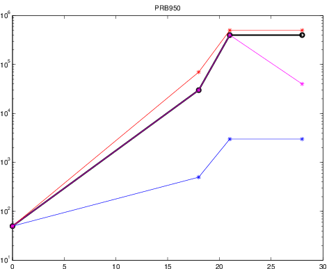
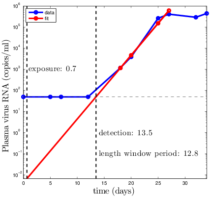
Simplest model
- Linear regression
- Extrapolate to the left until y=inoculum size
- Read off time of exposure
Mathematical Model
Simplest version: Fit linear regression, extrapolate
Mathematical Model
Simplest version:
Fit linear regression, extrapolate
Major shortcomings of linear regression:
- HIV infection is a stochastic event!
- Viral growth stochastic
- Most exposures do not lead to infection
Only 1/100-1/1000 (depending on exposure)
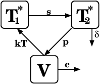
Stochastic model
Simplest stochastic analogue: Birth-death process

V \rightarrow V+1
Birth rate:
V \rightarrow V-1
Clearance rate:
Leads to exponential growth with rate b-c
Birth-death process
- Average growth = [birth] - [clearance]
- [clearance] = literature value (known)
- [birth] = [clearance] + [fitted average growth]
t = 0
N = INOCULUM_SIZE

while N < DETECTION_LIMIT:
    # Time to next event is exponentially distributed
    t += EXP(bN+cN)

    # Likelihood of event is proportional to reaction rates
    if RAND(0,1) < (b/b+c):
        # birth event
        N = N+1
    else:
        # clearance event
        N = N-1

return t
Birth-death process
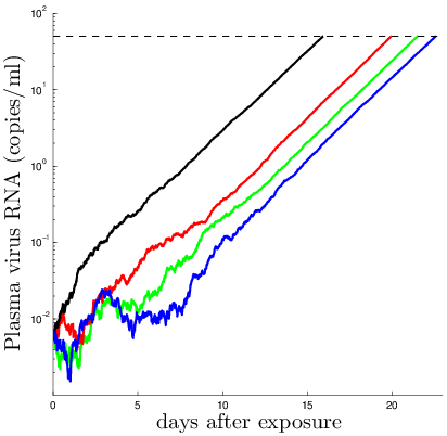
- Run simulations many times, for each growth rate
- Obtain distribution of length of window period
Technical: Avoid simulations
Instead of millions of Gillespie simulations, my research group found a way to calculate pdfs semi-analytically
- Much faster to compute
- Allows valuable insight
- Beautiful application of complex analysis :)
Technical: Avoid simulations
P(v, v_0, t) = Prob(V(t)=v\,|\,V(0)=v_0)
Set
\frac{d}{dt}P(v, v_0, t) = b(v-1)P(v-1, v_0, t) + c(v+1)P(v+1, v_0, t) - (b+c)vP(v, v_0, t)
Then we can easily derive the Master equation (balance equation)
v-1 and single birth
v+1 and single clearance
Leave state v by birth or clearance event
Knowing P means understanding everything!
Technical: Avoid simulations
\frac{d}{dt}P(v, v_0, t) = b(v-1)P(v-1, v_0, t) + c(v+1)P(v+1, v_0, t) - (b+c)vP(v, v_0, t)
P(v, v_0, t) = Prob(V(t)=v\,|\,V(0)=v_0)
Set
A little helper: The probability generating function
G(v_0, t, z) = \sum_v P(v, v_0, t)z^v
\frac{\partial}{\partial t}G(1, t, z) = b(G(1, t, z))^2 + c - (b+c)G(1, t, z)
G(1, 0, z) = z
Master equation: infinitely many ODEs!
Use branching property to derive single ODE
Technical: Avoid simulations
P(v, v_0, t) = Prob(V(t)=v\,|\,V(0)=v_0)
Set
Key observations:
P(v, v_0, t) = \frac1{v!}\left.\frac{\partial^v G(v_0, t, z)}{\partial z^v}\right|_{z = 0}
\frac{\partial}{\partial t}G(1, t, z) = b(G(1, t, z))^2 + c - (b+c)G(1, t, z)
G(v_0, t, z) = \sum_v P(v, v_0, t)z^v
G(v_0, t, z) = (G(1, t, z))^{v_0}
(branching property)
Technical: Avoid simulations
P(v, v_0, t) = Prob(V(t)=v\,|\,V(0)=v_0)
Set
P(v, v_0, t) = \frac1{v!}\left.\frac{\partial^v G(v_0, t, z)}{\partial z^v}\right|_{z = 0}
G(v_0, t, z) = \sum_v P(v, v_0, t)z^v
Instead of taking millions of derivatives (numerically unstable)...
...use Cauchy's integral formula!
f^{(n)}(0) = \frac{n!}{2\pi i} \oint_\gamma \frac{f(z)}{z^{n+1}}dz
Technical: Avoid simulations
P(v, v_0, t) = Prob(V(t)=v\,|\,V(0)=v_0)
Set
G(v_0, t, z) = \sum_v P(v, v_0, t)z^v
f^{(n)}(0) = \frac{n!}{2\pi i} \oint_\gamma \frac{f(z)}{z^{n+1}}dz
P(v, v_0, t) = \frac1{2\pi}\int_0^{2\pi} G(v_0, t, e^{i\varphi})\,e^{-iv\varphi}\,d\varphi
- Integration is numerically stable
- Resulting pdf for P is exact (Gillespie algorithm only gives approximation)
The hook is the hook
- How long is the window period?
- Given a negative HIV test t days after possible exposure, how likely is an infection?
- When to schedule second, confirmatory test?
Regardless of the method for the computation (Gillespie or semi-analytic), one major flaw remains:
HIV infection is very unlikely (0.1%-1%), but all observed patients became infected!
Extremely biased training set!
Maybe the virus was initially just "lucky" to grow faster than average!?
The hook is the hook
Heads: +1.1 points
Tails: -1 point
A) Start with 20 points
B) Start with 1 point
Lose when <= 0 points
The hook is the hook
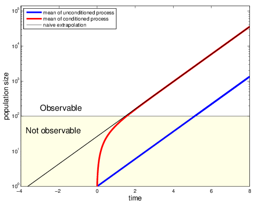
P(V(t) = v\,|\,V(0)=v_0, \color{red}{V(\infty) \neq 0})
Fit conditioned process to match the bias in the data
Virus not spontaneously cleared
Using Bayes rule and Markov property
P(V(t)=v\,|\,V(0)=v_0, V(\infty)\neq 0) = P(v, v_0, t)\frac{P(V(\infty)\neq 0\,|\,V(0) = v)}{P(V(\infty)\neq 0\,|\,V(0) = v_0)}
= P(v, v_0, t)\color{red}{\frac{1-q^v}{1-q^{v_0}}}
where q is likelihood that exposure by single virion leads to infection
The hook is the hook
Results
For actual risk calculations, replace b with more detailed model of viral replication
Fit unconditioned and conditioned model to patient data, assuming different risk scenarios
Results
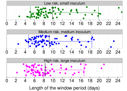
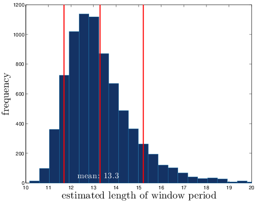
Distribution of the length of the window period
Due to hook: Shorter than previously expected!
Results
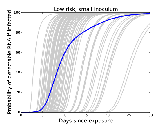
If infected: Averaged likelihood of detectable viral load at time t
Results
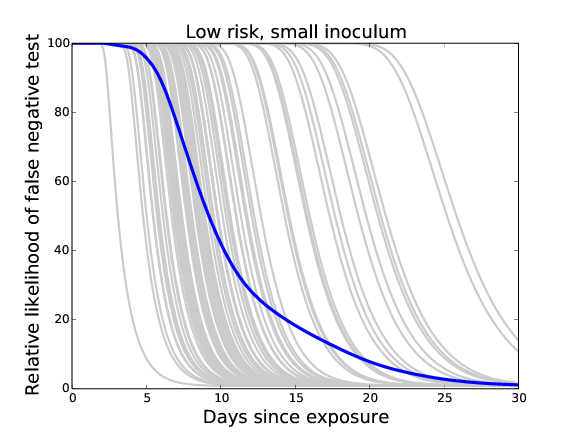
Likelihood of infection given a negative test at time t
days of neg test --- remaining risk
5.2 --- 0.475%
5.9 --- 0.450%
7.2 --- 0.375%
9.2 --- 0.250%
12.8 --- 0.125%
18.8 --- 0.050%
22.2 --- 0.025%
Summary
- Extracted and combined early viral load growth rates from various datasets
- Developed solid mathematical framework that is superior to previous methods
- Showed that excluding stochastic effects may lead to overestimation of length of window period
- Quantified uncertainty of early negative HIV test
- Gave recommendations to clinicians that help to find and treat real infections sooner
Future Work
- Help clinicians communicate stochastic results
- Include uncertainty from different HIV tests
- Specify model for different types of exposure
- Incorporate PEP and PrEP
- Confirm stochastic growth predictions with other data (eg. non-human primates, epidemics) and in experiments (eg. E. coli)
- Include information about the number of founder strains
Thank you!
Other PhD work
- Pre- and Post-Exposure Prophylaxis in early HIV infection
- Engineering a new anti-Malaria agent
- Math Education Resources
PrEP and PEP in early HIV
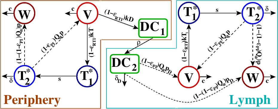
- Mathematically similar tools
- Trojan horse theory for dendritic cells
- Reverse transcriptase inhibitors better than protease inhibitors
- 2 weeks PrEP about as good as current recommendation of 4 weeks
Malaria
Built on Nature paper:
Engineering anti-malaria agent that stops onwards transmission in mosquitoes
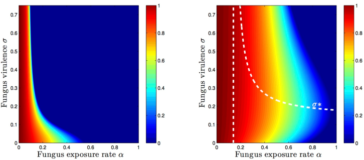
Trade-off between virulence and environmental effect
Math Education Resources
Lead to of volunteers to build free webapp with 1500 solutions to previous UBC Math exam questions
- One-vs-all SVC to predict topic of a newly added question (NLP)
- Recommendation algorithm to suggest next question based on course, peers, and difficulty
Stochastic Models of Early HIV Infection
By Bernhard Konrad