Control Synthesis & BRS Maximization using Occupation Measures and LMI Relaxations
Bernhard Paus Graesdal
6.7230 Algebraic Techniques & Semidefinite Optimization
Class project
- Based on the work by Majumdar et al.,
- As well as several other papers by:
- Henrion
- Korda
- Lasserre
- Han
- ++
Attributions
Problem Formulation
1. Problem Statement
\dot x(t) = f(t, x(t)) + g(t, x(t)) u(t,x(t))
We define bounding set, target set, and input sets:
\newcommand\Set[2]{\{\,#1\mid#2\,\}}
\begin{aligned}
x(t) \in X &:= \Set{x \in \mathbb{R}^n}{g_{X_i}(x) \geq 0 \, X_i = 1, \ldots, n_X}, \\
x(T) \in X_T &:= \Set{x \in \mathbb{R}^n}{g_{T_i}(x) \geq 0 \, X_i = 1, \ldots, n_T}, \\
u(t, x) \in U &:= [-1, 1]^m,
\end{aligned}
Consider control-affine dynamics:
1. Problem Statement
\newcommand\Set[2]{\{\,#1\mid#2\,\}}
\begin{aligned}
\mathcal{X}(u) := \Set{ x_0 \in \mathbb{R}^n}{\exists \ x \ \text{s.t.}& \\
\ x(0) &= x_0, \, x(T) \in X_T,
\\
\dot x (t) &= f(t,x(t)) + g(t, x(t)) u(t,x(t)), \\
x(t) &\in X, \, \forall t \in [0, T]},
\end{aligned}
Define Backwards Reachable Set (BRS):
(Same as the Region of Attraction (ROA))
1. Problem Statement
- Our goal is to find \(u^*\) that maximizes "size" of \( \mathcal{X} \)
- Denote by \( \lambda \) the Lebesgue measure
- Our problem:
\begin{aligned}
\max_{u} \quad& \lambda(\mathcal{X}(u)) \\
\text{subject to} \quad& u \in U
\end{aligned}
for \( \mathcal{X}(u) \) as defined on previous slide
2. Occupation Measures
Nonlinear ODE in \( t, x(t), u(t) \) \( \rightarrow \) Linear PDE in measures
\dot x(t) = f(t, x(t)) + g(t, x(t)) u(t,x(t))
\delta_T \otimes \mu_t =
\delta_0 \otimes \mu_0 +
\mathcal{L}_f' \mu +
\mathcal{L}_g' \sigma^+ -
\mathcal{L}_g' \sigma^-
\downarrow
Result:
Idea:
2. Occupation Measures
\begin{aligned}
\mu(A \times B \mid x_0) &:= \int^T_0 \mathbb{I}_{A\times B}(t, x(t \mid x_0)) dt, \\
&A \in \mathcal{B}([0,T]), \; B \in \mathcal{B}(X)
\end{aligned}
- Define occupation measure as
(\( \mathcal{B}(S) \) is the \(\sigma\)-algebra of set \(S\))
"How much time is spent by a system trajectory starting at \(x_0\) in a set \(A\times B\)"
- Key point: Time-integration over a system trajectory \( \iff\) integration w.r.t \(\mu\)
2. Occupation Measures
\mu(A \times B) := \int_X \mu(A \times B \mid x_0) \mu_0(dx_0),
- Let \(x_0\) be a random variable, distributed according to \( \mu_0 \)
- Define average occupation measure
- And target measure
\mu_T(B) := \int_X \mathbb{I}_{B}(x(T \mid x_0) \mu_0(dx_0)
"How much time is spent in a set \(A\times B\) on average"
"How much of the state-space ends up in \(B\) on average"
2. Occupation Measures
\begin{aligned}
\sigma_j(A \times B) &:= \sigma_j^+(A \times B) - \sigma_j^-(A \times B) \\
&=
\int_{A} \int_{B} u_j (t, x(t)) \mu(dt, dx)
\end{aligned}
- Define signed control measure as
2. Occupation Measures
Nonlinear ODE \(\rightarrow\) linear PDE
- Look at time-integration of a test function \(v(t,x)\) over a system trajectory
- Integrate w.r.t to \( \mu_0 \)
- \( \implies \) a relationship between measures!
\int_X v(T,x) \mu_T(dx) = \int_X v(t, x) \mu_0(dx)
+ \int_0^T \int_X [\mathcal{L}_f v(t,x) + \mathcal{L}_g v(t,x) u(t,x) ] \mu(dt, dx)
\delta_T \otimes \mu_t =
\delta_0 \otimes \mu_0 +
\mathcal{L}_f' \mu +
\mathcal{L}_g' \sigma^+ -
\mathcal{L}_g' \sigma^-
\Updownarrow
"Controlled Lioville's Equation"
2. Occupation Measures
Nonlinear ODE \(\rightarrow\) linear PDE
- Investigate time-integration of a test function \(v(t,x)\) over a system trajectory:
\begin{aligned}
v(T, x(T \mid x_0)) &= v(0, x_0)
+ \int^T_0 \dot v(t, x(t \mid x_0)) dt \\
&= v(0, x_0) +
\int^T_0 [ \mathcal{L}_f v(t, x(t \mid x_0)) + (\mathcal{L}_g v(t,x(t \mid x_0))) u(t, x(t, \mid x_0)) ] dt
\end{aligned}
\int_X v(T,x) \mu_T(dx) = \int_X v(t, x) \mu_0(dx)
+ \int_0^T \int_X [\mathcal{L}_f v(t,x) + \mathcal{L}_g v(t,x) u(t,x) ] \mu(dt, dx)
- Idea: Integrate with respect \(\mu_0\)
Relation w.r.t to measures
\(\uparrow\)
2. Occupation Measures
- Must hold for all test functions \( v(t,x) \)
- Rewrite as relation between operators:
- Controlled Lioville's Equation
- A linear PDE in measures!
\delta_T \otimes \mu_t =
\delta_0 \otimes \mu_0 +
\mathcal{L}_f' \mu +
\mathcal{L}_g' \sigma^+ -
\mathcal{L}_g' \sigma^-
\int_X v(T,x) \mu_T(dx) = \int_X v(t, x) \mu_0(dx)
+ \int_0^T \int_X [\mathcal{L}_f v(t,x) + \mathcal{L}_g v(t,x) u(t,x) ] \mu(dt, dx)
3. Maximizing the BRS
- Represent BRS as \( \text{spt}(\mu_0) \)
- Maximize BRS as: enforce \( \mu_0 \leq \lambda \), maximize \( \mu_0(X) \)
\begin{aligned}
\sup \quad& \mu_0(X) \\
\text{subject to} \quad&
\delta_T \otimes \mu_t -
\delta_0 \otimes \mu_0
=
\mathcal{L}_f' \mu +
\mathcal{L}_g'(\sigma^+ - \sigma^-) \\
& \sigma^+ + \sigma^- + \hat \sigma = \mu \\
& \mu_0 + \hat \mu_0 = \lambda
\end{aligned}
- Inifinite-dimensional LP over measures
- Measures are nonnegative
- Their supports model bounding set and target set
3. Maximizing the BRS
- Dual problem in space of continuous functions
\begin{aligned}
\inf \quad& \langle \lambda, w \rangle \\
\text{subject to} \quad&
\mathcal{L}_f v + 1^\intercal p \leq 0, \quad \forall t, x \in [0,T] \times X \\
\quad& p \geq 0, \quad \lvert \mathcal{L}_g v \rvert \leq p, \quad \forall t, x \in [0,T] \times X \\
\quad& w \geq 0, \quad \forall x \in X \\
\quad& w \geq v(0, \cdot) + 1, \quad \forall x \in X \\
\quad& w(T, \cdot) \geq 0, \quad \forall x \in X_T
\end{aligned}
- Decision variables: \( v(t,x), p_j(t,x), w(x) \)
4. SOS Relaxation
\begin{aligned}
\inf \quad \sum_\alpha w_\alpha \lambda_\alpha & \\
\text{subject to} \quad
-\mathcal{L}_f v - 1^\intercal p &\in Q_{2k}([0,T]\times X) \\
\quad p, p - \lvert \mathcal{L}_g v \rvert &\in Q_{2k}([0,T]\times X) \\
\quad w &\in Q_{2k}(X) \\
\quad w - v(0, \cdot) - 1 &\in Q_{2k}(X) \\
\quad w(T, \cdot) &\in Q_{2k}(X_T)
\end{aligned}
- We solve this problem
- Equivalent to solving the k-th step of Lasserre's Hierarchy on the primal side
- Relax the dual using SOS:
5. Extracting a controller
M_k(y_{k,\mu}) \text{vec}(u_j) =
y_{k, \sigma^+_j} - y_{k, \sigma^-_j}
- Bad news: don't get \(u\) directly
- Solve linear system for coefficients of \(u\):
- \(M_k\) generally only PSD
- Use generalized inverse \(\rightarrow\) Numerical issues
Numerical Results
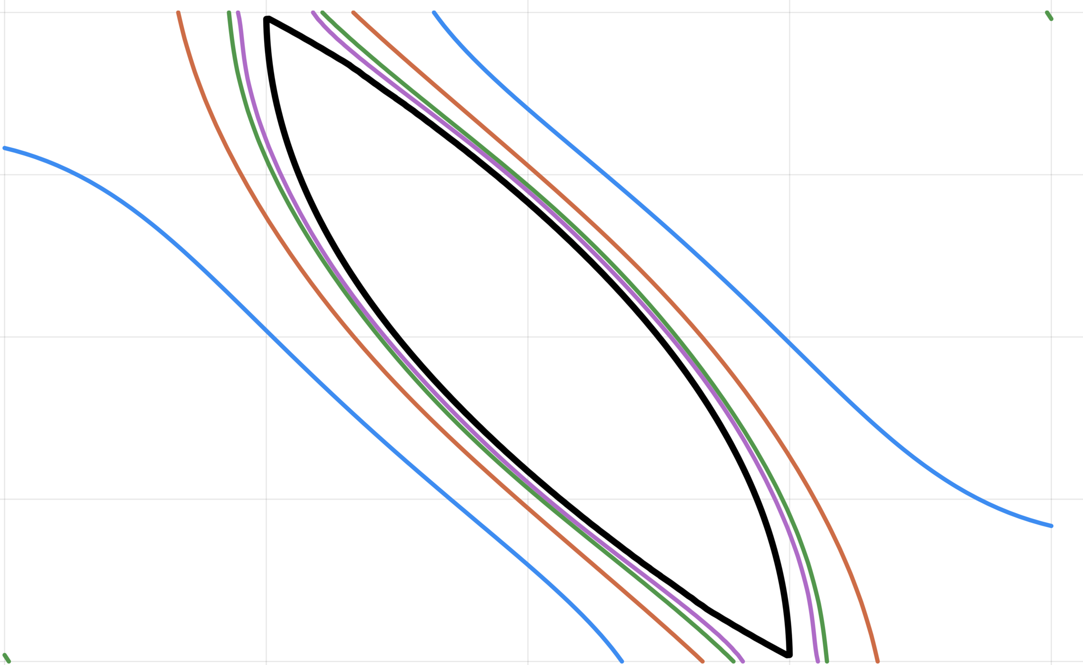
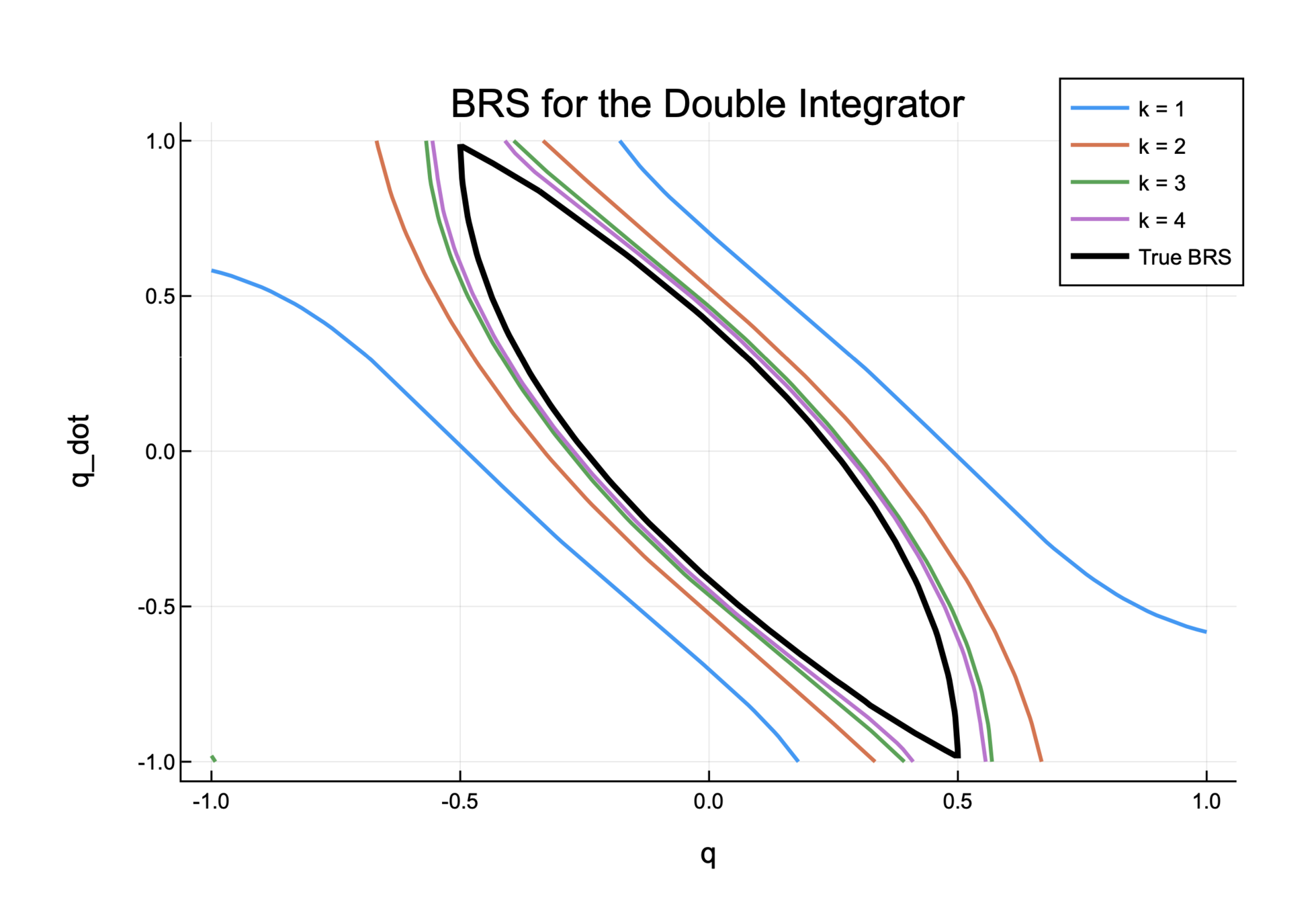
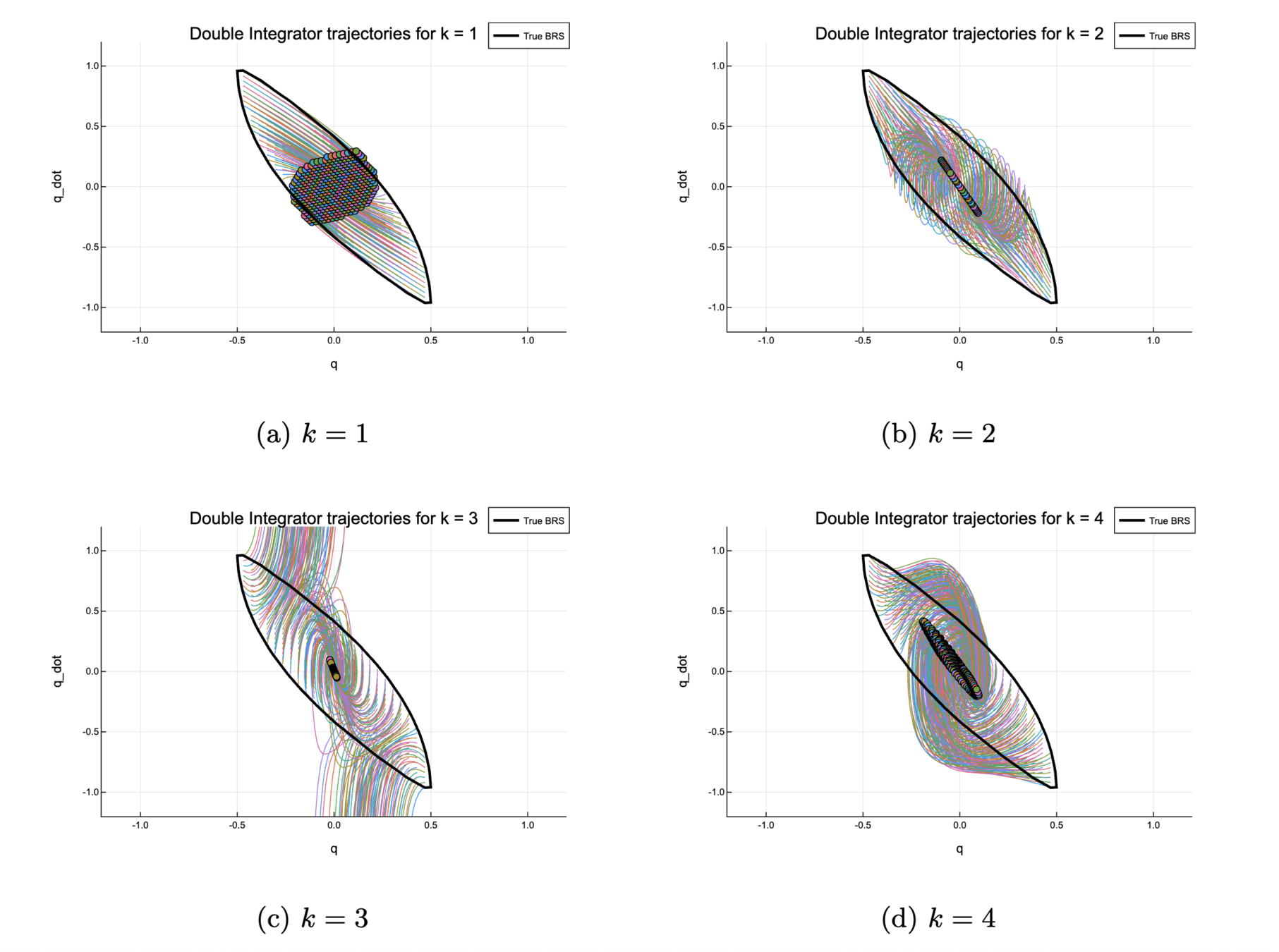
1. Double Integrator
\newcommand\Set[2]{\{\,#1\mid#2\,\}}
\begin{aligned}
\dot x_1 &= x_2 \\
\dot x_2 &= u \\
\end{aligned}
\newcommand\Set[2]{\{\,#1\mid#2\,\}}
\begin{aligned}
X &= \Set{x \in \mathbb{R}^2}{-1 \leq x \leq 1} \\
X_T &= \Set{x \in \mathbb{R}^2}{-\epsilon \leq x \leq \epsilon}, \quad \epsilon = 0.001 \\
U &= [-1,1]
\end{aligned}
- Dynamics:
- Sets:
1. Double Integrator
Outer-approximation to BRS
1. Double Integrator
Synthesizing a stabilizing controller with LSE
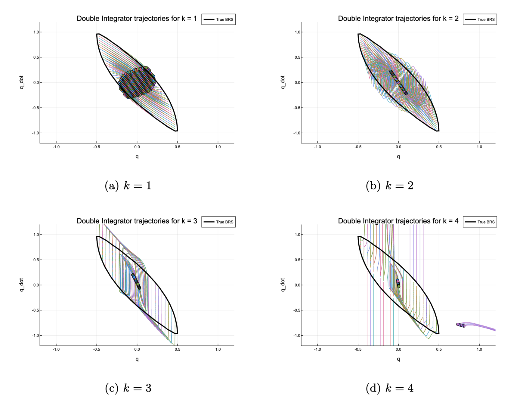
1. Double Integrator
Adding regularization
1. Double Integrator
Look at numerical properties
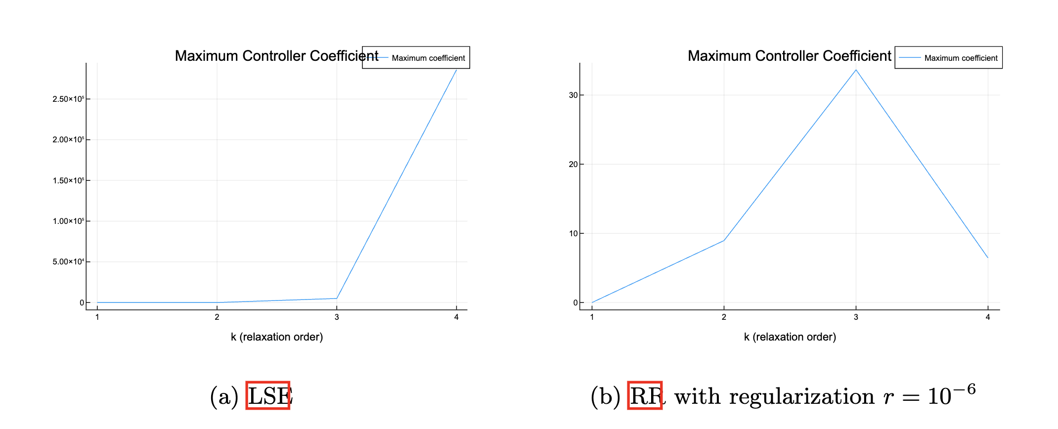
M_k(y_{k,\mu}) \text{vec}(u_j) =
y_{k, \sigma^+_j} - y_{k, \sigma^-_j}
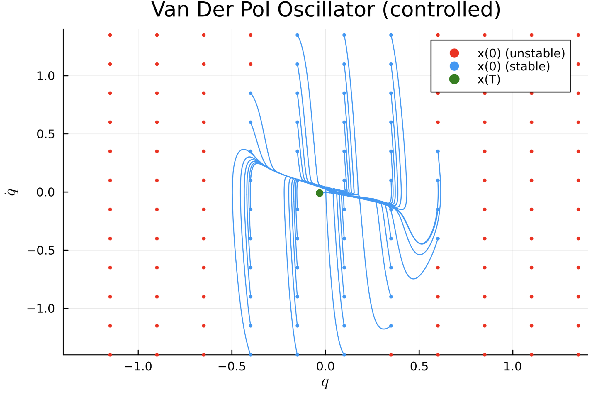
2. Van der Pol Oscillator
\begin{aligned}
\dot x_1 &= -2 x_2
\\
\dot x_2 &= 0.8 x_1 + 10 (x_1^2 - 0.21) x_2 + 0.1 u
\end{aligned}
- Dynamics:
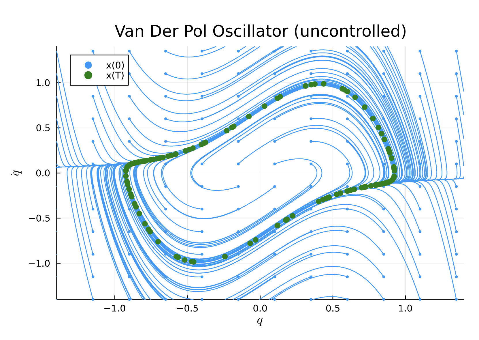
- Uncontrolled phase-space plot:
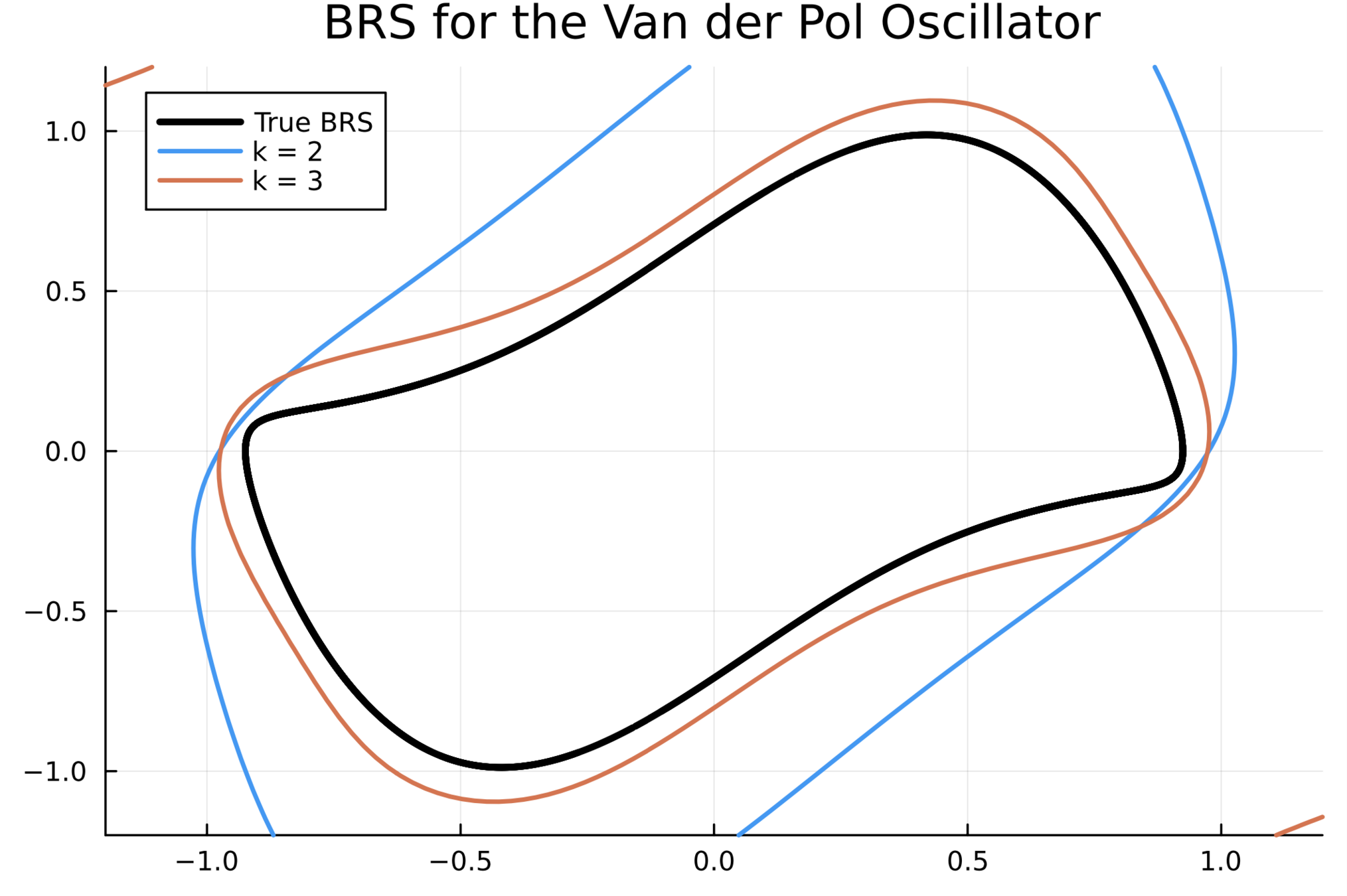
2. Van der Pol Oscillator
Outer-approximation to BRS
2. Van der Pol Oscillator
Synthesizing a stabilizing controller
Discussion & Conclusion
Key takeaways
- Appealing on a theoretical level
- Deals with any nonlinear, polynomial system
- Has extensions to the hybrid and discrete case
- Numerical issues when extracting the controller
- Numerical issues for big SOS problems
Future Work
- Output feedback
- Hybrid systems
- Test "pure" Optimal Control instead of BRS
Controller Synthesis for Maximization of the Backwards Reachable Set using Occupation Measures and LMI Relaxations
By Bernhard Paus Græsdal


