Statistical characterization of SAPS velocities
B. S. R. Kunduri, J. B. H. Baker, J. M. Ruohoniemi, S. G. Shepherd, P. J. Erickon, A. J. Coster and E. G. Thomas
Introduction - SD SAPS Location model
Kunduri et al [2017], under review.
Introduction - Velocity characterization
Kunduri et al [2017], under review.
Problem statement
-
In Kunduri et al., [2017] (under review), we
- developed SuperDARN based SAPS location model
- discussed SAPS speeds using gridded line-of-sight velocities assuming SAPS were perfectly westwards.
-
A detailed characterization of SAPS velocities is required to complete the SAPS model. In this study
- we analyze variations in SAPS flow direction with MLT.
- we analyze mean SAPS velocities at different Dst bins and MLTs.
- we derive kernel density estimates of SAPS velocities.
Traditional L-shell fitting approach [Clausen et al., 2012]
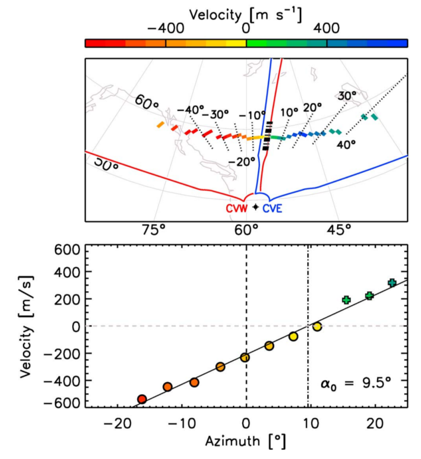
- Clausen et al [2012] approach was to derive one L-shell fit for each radar pair. The approach was ideally suitable for case studies.
- Not directly adaptable to statistical studies.
- Three L-shell fit velocities (3 radar pairs) for data spanning more than 7 hours in MLT would be under utilization of resources.
- The first step is make L-shell fitting applicable to statistical studies.
Optimized use of regions with "good" scatter
- Instead of one velocity for each radar pair. We search the entire "map" to detect locations where L-shell fitting can be applied (irrespective of radars).
- Regions where common volume measurements are available (highlighted above) are especially suited for applying L-shell fitting technique.
Identify all regions with "good" scatter
- Apply a standard grid over SAPS observations.
- Each cell in the grid is 1 hour MLT, 0.5 degrees MLAT (SAID features have narrow latitudinal range).
- Cells with "good" scatter will:
- have measurements with l-o-s azimuth range > 35.
- Atleast have 3 unique azimuth measurements.
- When fitting a sinusoid, determined SAPS azimuth should be within -90 +/- 20 degrees.
- Fitting error should be less than 25%.
- NOTE : L-o-s velocities below 150 m/s are discarded.
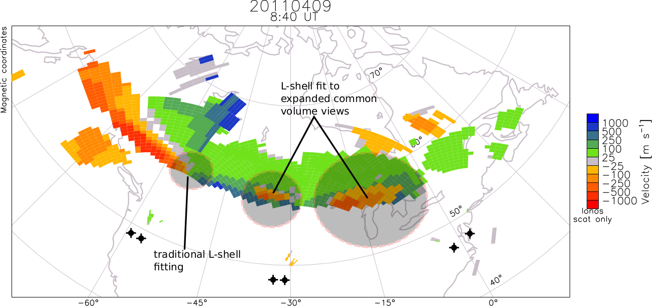
L-shell map (April 9, 2011 0840 UT)
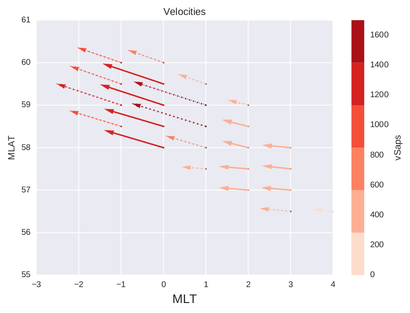
- Solid lines indicate velocities where "good" L-shell fit could be derived,
- Dashed lines indicate velocities whose directions were assumed to be same as the nearest "good" fit.
- Results are comparable to Clausen et al, [2012].
- The L-shell map approach is suitable for statistical studies. - 1) results are standardized for all events. 2) not impacted by data availability at radar pairs.
L-shell map movie : Apr-9-2011
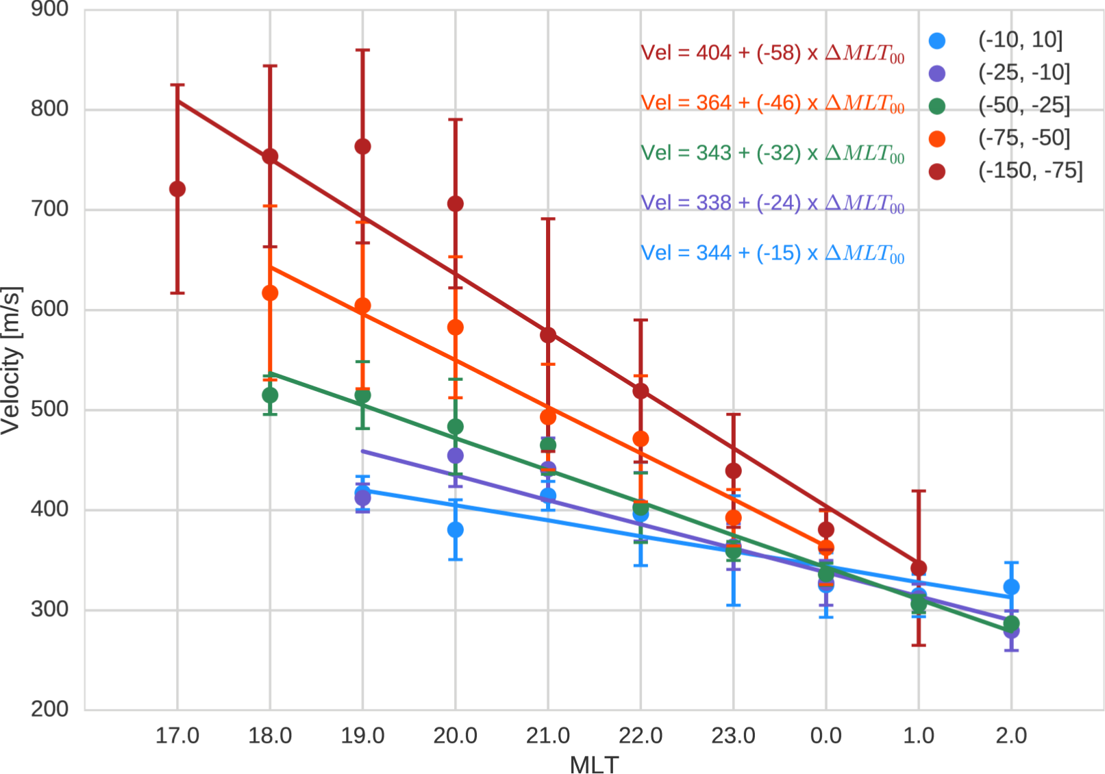
Mean velocities by Dst bins
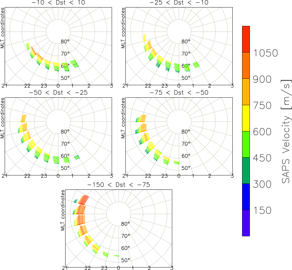
- Mean SAPS velocities at each Dst bin.
- Velocities are higher in the dusk sector.
- Velocities are higher at lower Dst levels.
Azimuths (and linear fits) by Dst bins
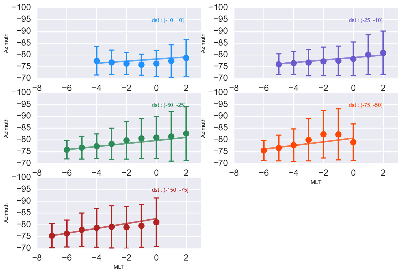
- Mean and std. dev. of SAPS velocity directions at different Dst bins. -90 is perfectly westwards. The solid lines represent a linear fit to mean azimuths.
- Flow direction becomes increasingly polewards towards dusk. Indicative of SAPS merging with auroral flows eventually? The pattern is also observed (not discussed) in Clausen et al [2012] event.
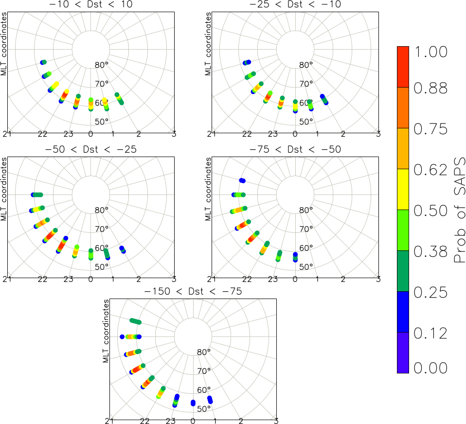
Kernel density estimates of velocities
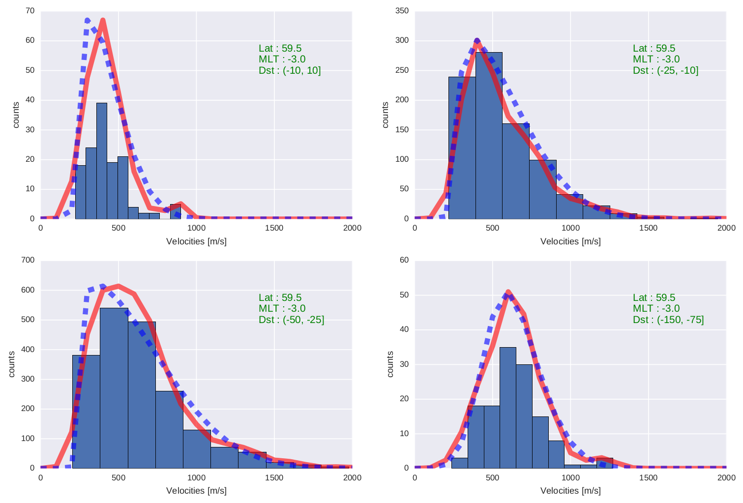
- The Figure presents histograms, kernel density estimates (red) and fitted skewed gaussian curves (dashed blue) for SAPS velocities for different Dst bins at a selected location.
- Skewed gaussian appears to be a better fit for the KDEs (after trying several others).
- The likelihood of observing higher velocities increases with geomagnetic activity.
- With decreasing Dst gaussian curve changes from right skewed to left skewed.
Modeling the kernel density estimates
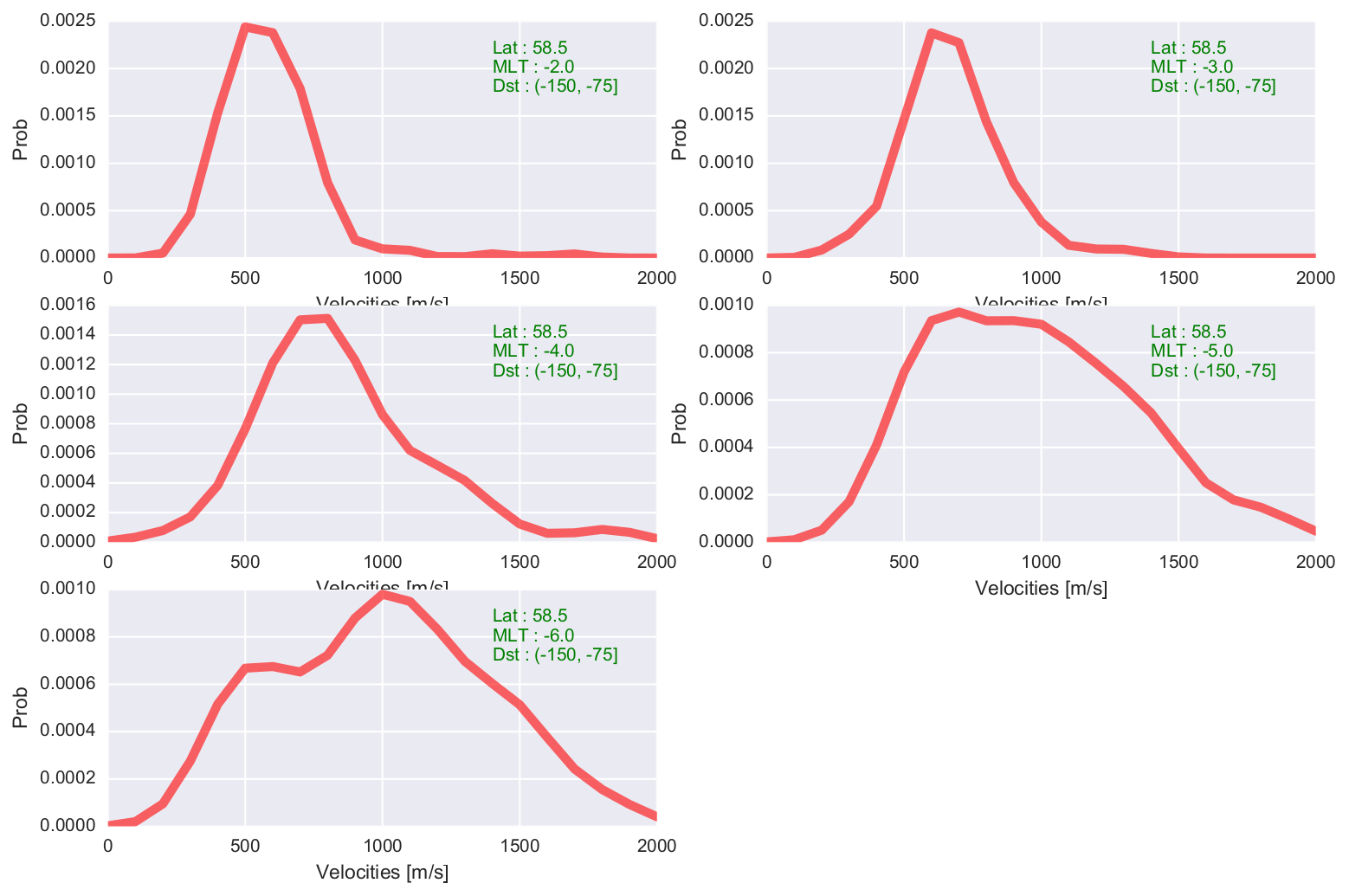
- Figure shows KDEs of velocities for lowest dst bin at different MLTs.
- Likelihood of observing higher velocities increases near dusk.
- Each KDE can be modeled separately, but a universal model (function of Dst, MLAT, MLT) like SAPS location model is difficult.
Conclusions
- Used L-shell fitting to estimate SAPS velocities
- The mean SAPS velocities increased as we move towards dusk and at higher disturbance levels.
- Flow direction was more polewards near dusk than near mid-night.
- Kernel density estimates of velocities at a given location and dst-bin suggest a skewed gaussian distribution of velocities.
- Developing a dst and geomagnetic location based common model is proving difficult. Tried different fits/distributions - skewed gaussian, rayleigh etc.
L-shell fitting
By Bharat Kunduri


