Electron Density Reconstruction in the Ionosphere
Brian Breitsch
Advisor: Dr. Jade Morton

TEC, tomography, assimilation, GNSS occultations, spherical symmetry
A vague, uninformed, and somewhat rambling overview of
Outline
- TEC
- tomography
- ionosonde/ISR
- radio occultation
- spherical symmetry inversion
- derivation
- results
- limitations
- other imaging methods using RO
Electron Density
and Reconstruction
- electron density is the image
- total electron content is the typical observable
- also , ,
- is the path integral of
N_e
TEC
TEC
N_e
VTEC
STEC
LTEC
Austen et. al. 1988
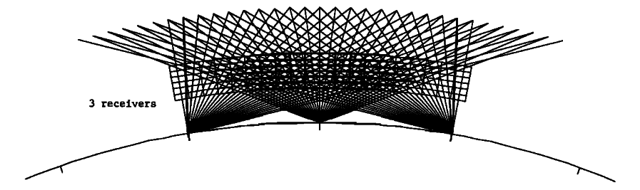
three receiver simulation geometry
Ionospheric Imaging Using Computerized Tomography
- simulation study
- 2D plane
- suggests feasibility of ionosphere tomography
- indicates poor vertical resolution
Yeh and Raymund 1991
Limitations of Ionospheric Imaging by Tomography
- detailed mathematical analysis
- impulse response methods
- quantitative results for resolution
- affirms poor vertical resolution

Tomography Successes
- early success with polar orbiting beacons
- NNSS (Navy Navigation Satellite System)
- near-polar orbit at 1000km


Na et. al. 1990 imaging of ionosphere trough
Tomography Successes
- Yizengraw et. al. 2003
-
Tomographic reconstruction of the ionosphere using ground-based GPS data in the Australian region
-
GPS satellites in 2D geometry
-
showed ionospheric trough during geomagnetic storm

Tomography Successes
- many others
- most using a priori information
- model-based background
- many using regularization contraints
- orthonormal basis functions
- spherical harmonics
- model-based functions
- Chapman
- DGR (Giovanni and Radiacella, Radiacella & Zhang 1995)
- orthonormal basis functions

tomographic image and EISCAT verification, Mitchel et. al. 1997
Problems
- 2D plane assumption invalid
- poor vertical resolution
- poor temporal resolution with GPS satellites
- ill-posed inverse problem
- especially in 3D
- need for regularization
- need for more data
Ionosondes and ISRs
advantages
- provide high-resolution vertical information
- on-demand (ish) sounding
disadvantages
- size
- cost to build/operate
- restricted location
- bottomside profile only for ionosondes

Radio Occultations
- Earth limb sounding of TEC (LTEC)
- provide information with good vertical resolution
- even, global distribution of soundings

- useful for tomography and model assimilation
- complementary to ground-GNSS geometry

Reconstruction
radio occultation data can stand on its own
- spherical symmetry assumption for provides sufficient regularization
- resulting inverse problem is well-defined
- solution to Abel inversion is least-squares solution to corresponding system
N_e
y = Ax
A
upper triangular
Reconstruction
assuming spherical symmetry

dx = \frac{r}{\sqrt{r^2 - y^2}} dr
r = \sqrt{y^2 + x^2}
F(y) = \int_{-\infty}^{\infty}\frac{rf(r)}{\sqrt{r^2 - y^2}} dr
Reconstruction
layers

- assume varies linearly between layers
N_e
N_i(r) = N(p_{i-1}) + \frac{N(p_{i}) - N(p_{i-1})}{p_{i} - p_{i-1}} (r - p_{i-1})
between and layers, define election density:
i^{th}
i-1^{th}
\Rightarrow N_{i}(r) = a_{i} + b_{i} r
Reconstruction
TEC observation expression
- TEC typically defined in TECU:
- redefine as:
1e16 \text{ electrons} / m^2
T(p_i) = 1e16 \cdot TEC(p_i)
p_i
where is the impact parameter for layer
i
i = M - 1, ..., 0
M = \text{ number of layers}
T(p_i) = \sum_{k=1}^m 2 \int_{p_{i+k-1}}^{p_{i+k}} \frac{rN_{i+k}(r)}{\sqrt{r^2 - p_i^2}}dr
m = M - i
Reconstruction
solving integrals
- plug in linear expression:
- solve integrals
N_{i}(r) = a_i + b_i r
\int_{p_{i+k-1}}^{p_{i+k}} \frac{rN_{i+k}(r)}{\sqrt{r^2 - p_i^2}}dr
\int \frac{r}{\sqrt{r^2 - p^2}}dr \Rightarrow \sqrt{r^2 - p^2}
\int \frac{r^2}{\sqrt{r^2 - p^2}}dr \Rightarrow \frac{1}{2} \left[ r\sqrt{r^2 - p^2} + p^2 \ln\left|\frac{1}{p}\left(r + \sqrt{r^2 - p^2} \right)\right| \right]
Reconstruction
expand solution
\int_{p_{i+k-1}}^{p_{i+k}} \frac{rN_{i+k}(r)}{\sqrt{r^2 - p_i^2}}dr
\rho_{i,k} = \frac{ \alpha_{i,k} - \alpha_{i,k-1} }{p_{i+k} - p_{i+k-1}}
\sigma_{i,k} = \frac{ p_{i+k} \alpha_{i,k} - p_{i+k-1} \alpha_{i,k-1} }{2 p_i \left(p_{i+k} - p_{i+k-1}\right)} + \frac{p_i^2}{2\left(p_{i+k} - p_{i+k-1}\right)} \ln \left| \frac{ p_{i+k} + \alpha_{i,k} }{ p_{i+k-1} + \alpha_{i,k-1} } \right|
- define:
2\sum_{k=1}^m
\left[
N(p_{i+k-1}) \left( p_{i+k} \rho_{i,k} - \sigma_{i,k} \right)
-
N(p_{i+k}) \left( p_{i+k-1} \rho_{i,k} - \sigma_{i,k} \right)
\right]
T(p_i) =
\alpha_{i,k} = \sqrt{p_{i+k}^2 - p_{i}^2}
Reconstruction
group corresponding layers
\frac{T(p_i)}{2} =
N(p_i) (p_{i+1} \rho_{i,1} - \sigma_{i,1})
+ \sum_{k=1}^{m-1}
N(p_{i+k}) \left( p_{i+k+1} \rho_{i, k+1} - \sigma_{i, k+1} - p_{i+k-1} \rho_{i, k} + \sigma_{i, k} \right)
- N(p_{i+m})(p_{i+m-1} \rho_{i,m} - \sigma_{i,m})
Reconstruction
final expression
N(p_i) =
\frac{1}{p_{i+1}\rho_{i,1} - \sigma_{i,1}} \left[ \frac{T(p_i)}{2}
\right]
- \sum_{k=1}^{m-1} N(p_{i+k}) \left( p_{i+k+1} \rho_{i, k+1} - \sigma_{i, k+1} - p_{i+k-1} \rho_{i, k} + \sigma_{i, k} \right)
\left[
+ N(p_{i+m})(p_{i+m-1} \rho_{i,m} - \sigma_{i,m})
\right]
Reconstruction
top-layer density
N(p_i) = N(p_M)
- assume is constant for near
N(p_i)
p_i
p_M
then
T(p) = 2\int_p^{p_M} \frac{r N(p_M)}{\sqrt{r^2 - p^2}} dr = 2 N(p_M) \sqrt{p_M^2 - p^2}
= 2 N(p_M) \sqrt{(p_M + p)(p_M - p)}
\approx 2 N(p_M) \sqrt{2 p_M (p_M - p)}
perform fit of top few measurements to find
TEC
N(p_M)
Reconstruction
above-LEO
- subtract off for positive elevation angle
- usually
TEC
TEC

\approx 1-3 \ \ TEC
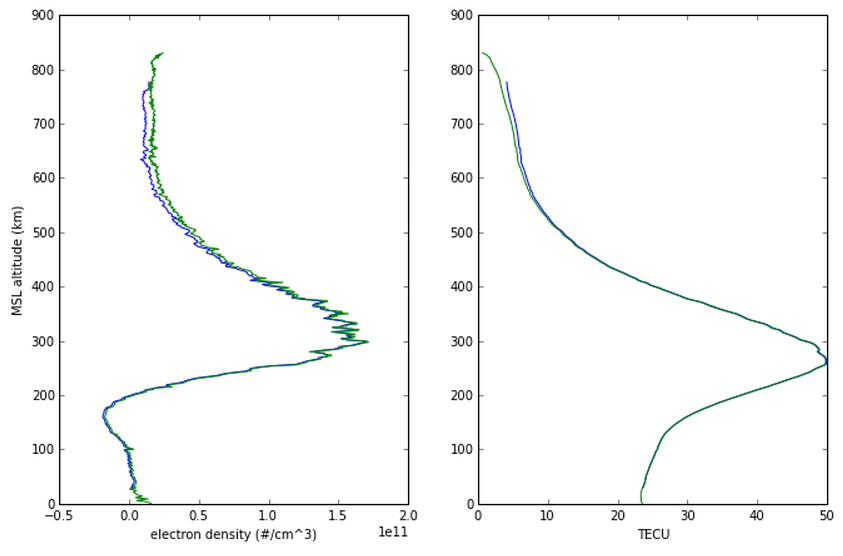
Results
no calibration

Results
DCB calibration (guess/fit)

Results
above-LEO calibration
Horizontal Gradients
Case: Ascension Island

- scintillation amongst GNSS satellites suggests horizontal gradients
- manifest through invalid electron density profile reconstruction
Horizontal Gradients
impact on spherical symmetry assumption
- Shaik et. al. 2013 does investigates impact of spherical symmetry assumption in ionospheric imaging
- found good correlation between horizontal gradients and profile retrieval error

VTEC modeled using NeQuick2 with hypothetical occultation tangent point overlay
Horizontal Gradients
Using VTEC to scale profile shape
<results from paper>
Other Methods
wave-theoretic
- use LEO orbit as synthetic aperture
- spectrum inversion
- addresses multipath concerns
- not relevant in ionosphere
- potentially very useful in troposphere


Jensen et. al. 2003 FSI simulation
Model Assimilation
- includes physics-based a priori model
- uses all data sources
- 4D imaging
Simply the most comprehensive and effective way to image the ionosphere.
Bust 2008 provides historical context for 2D tomography leading into 4D tomography/assimilation
Tomography/Assimilation
- Ionospheric Data Assimilation Three Dimensional (IDA3D)
- uses 3 dimensional variational data assimilation
- Regional Ionospheric Mapping and Tomography (RIMT)
- toolkit developed at Cornell, used in multiple studies
- everyone, everywhere, is/was doing ionosphere imaging
- Stanford
- Cornell
- University of California, Los Angeles
- University of Texas, Austin
- University of Calgary, Canada
- La Trobe University, Bundoora, Australia
- Wuhan University, China
- University of Wales, Aberystwyth, U.K.
Data Assimilation
IDA3D
- Bust et. al. 2007
- showed convective transport at polar cap
Proposal
Goal: to improve vertical ionosphere profile reconstruction using RO measurements w/o need for full-blown 3D/4D assimilative model?
- use IRI for contributions of top-layers in lower-layer reconstruction
- disadvantage: model could have significant bias
-
Yeh, K. C., and T. D. Raymund. "Limitations of Ionospheric Imaging by Tomography." Wiley Online Library. Radio Science
- Radicella, Sandro Maria, and Man-Lian Zhang. "The Improved DGR Analytical Model of Electron Density Height Profile and Total Electron Content in the Ionosphere." Annali Di Geofisica 38 (1995): 35-41.
- Montebruck, Oliver, and Eberhard Gill. "Ionospheric Correction for GPS Tracking of LEO Satellites." The Journal of Navigation, n.d. Web. 01 July 2015.
-
Mitchell, C. N., L. Kersley, J. A. T. Heaton, and S. E. Pryse. "Determination of the Vertical Electron-density Profile in Ionospheric Tomography: Experimental Results." Annales Geophysicae 15 (1997): 747-52.
-
Hernandez-Pajares, M., J. M. Juan, and J. Sanz. "Improving the Abel Inversion by Adding Ground GPS Data to LEO Radio Occultations in Ionospheric Sounding." Geophysical Research Letters - Wiley Online Library. Group of Astronomy and Geomatics, n.d. Web. 01 July 2015.
-
Garcia-Fernandez, Miquel, Manuel Hernandez-Pajares, Jose Miguel Juan-Zornoza, and Jaume Sanz-Subirana. "An Improvement of Retrieval Techniques for Ionospheric Radio Occultations." ResearchGate. Astronomy and Geomatics Research Group, n.d. Web. 01 July 2015.
-
Fremouw, E. J., and James A. Secan. "Application of Stochastic Inverse Theory to Ionospheric Tomography" Radio Science - Wiley Online Library. Radio Science, n.d. Web. 01 July 2015.
-
Bernhardt, P. A., K. F. Dymond, J. M. Picone, D. M. Cotton, S. Chakrabarti, T. A. Cook, and J. S. Vickers. "Improved Radio Tomography of the Ionosphere Using EUV/optical Measurements from Satellites." Radio Sci. Radio Science 32.5 (1997)
- Spencer, Paul S. J., Douglas S. Robertson, and Geral L. Mader. "Ionospheric Data Assimilation Methods for Geodetic Applications." (2005): n. pag. Web.
deck
By Brian Breitsch


