Improved Estimation of Ionosphere TEC Using Triple-Frequency GPS Signals
Brian Breitsch
Advisor: Dr. Jade Morton

- Background and Motivation
- Geometry-free Combinations
- ILS TEC Estimation
- Experiment
-
TEC Leveling
- VTEC Gradient-Mapping Method
- Results
- Conclusions / Future Work
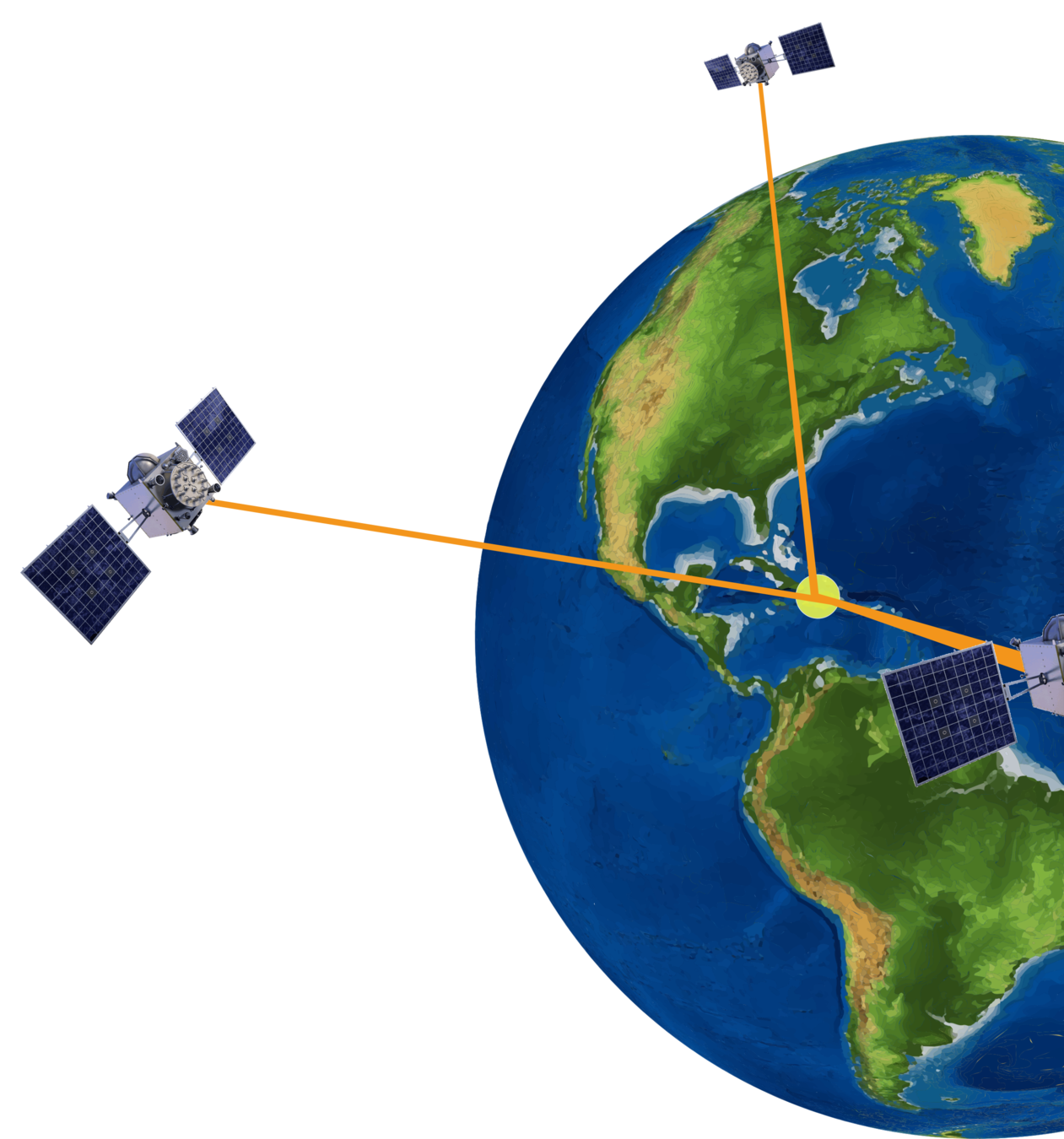
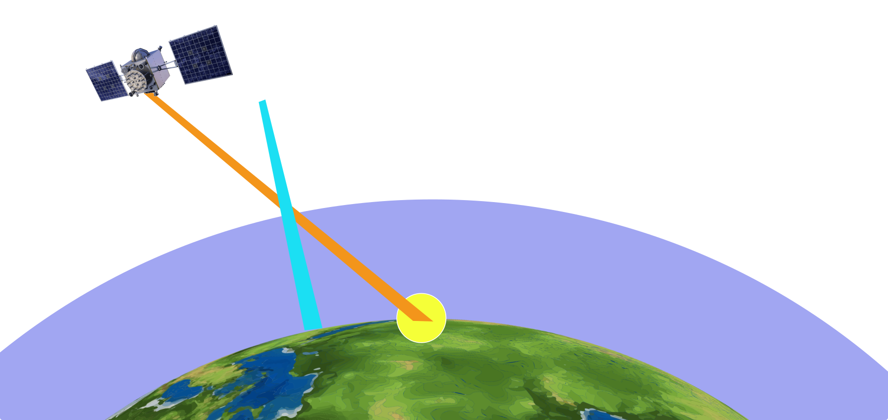
Ionosphere TEC
TEC = \int_{\text{rx}}^\text{sat} N_e(x) dx
ionosphere-induced range error for a particular satellite and carrier frequency
\approx \frac{f^2}{40.3\times 10^{16}}I_{S,f}
1st-order approx.
GNSS Observations
\rho_{S,f} = r_S + c\left( \Delta t_s - \Delta t_R \right) + T_S
+ b^\rho_{S,f} + b^\rho_{R,f} + I_{S,f} + M^\rho_{S,f} + \epsilon^\rho_{S,f}
\phi_{S,f} = r_S + c\left( \Delta t_s - \Delta t_R \right) + T_s
+ b^\phi_{S,f} + b^\phi_{R,f} - I_{S,f} + \lambda_f N_{S,f} + M^\phi_{S,f} + \epsilon^\phi_{S,f}
HARDWARE
BIAS
IONOSPHERE DELAY
CARRIER
AMBIGUITY
MULTIPATH EFFECTS
FREQUENCY INDEPENDENT EFFECTS
Previous Work
Dissertation by Justine Spitz focused on 3-frequency signal combinations allowing improved real-time resolution of carrier ambiguities and TEC estimation
L1CA
L2C
L5
linear combination
loss of information
TEC \approx \frac{\alpha_{f_i, f_j}}{40.3\times 10^{16}} \left( I_{S,f_i} - I_{S,f_j}\right)
What can we accomplish with one receiver and 3-frequency GPS measurements?
Most previous work in TEC estimation uses dual-frequency GNSS receiver
- large receiver networks
- physical / thin-shell / tomographic ionosphere model
Bias and Error Assumptions
b_{S,f}^\phi \approx b_{S,f}^\rho
b_{R,f}^\phi \approx b_{R,f}^\rho
assume no code-carrier bias
\Delta b_{S,f_i,f_j}, \ \Delta b_{R, f_i, f_j}
- receiver code-carrier bias usually compensated for by manufacturer
since we will use geometry free combinations, we only care about inter-frequency biases
(IFB)
E\left[ M_{f_i} M_{f_j} \right] \approx 0
M^\phi \ll M^\rho
multipath uncorrelated across different signals
carrier pseudorange noise / multipath is small compared to code
not true
\epsilon^\phi \ll \epsilon^\rho
\approx \text{constant}
over 1 day
Geometry-Free Combinations
\phi_{S,f_i} - \phi_{S,f_j} = \Delta b_{S,f_i,f_j} + \Delta b_{R,f_i,f_j} - \left(I_{S,f_i} - I_{S,f_j} \right)
+ \lambda_{f_i}N_{S,f_i} - \lambda_{f_j}N_{S,f_j} + M^\phi_{S,f_i} - M^\phi_{S,f_j} + \epsilon^\phi_{S,f_i} - \epsilon^\phi_{S,f_j}
\rho_{S,f} - \phi_{S,f} \approx 2I_{S,f} - \lambda_fN_{S,f} + M_{S,f}^\rho + \epsilon_{S,f}^{\rho}
\Delta ADR_{f_i,f_j}
CMC_f
Geometry-Free Combinations
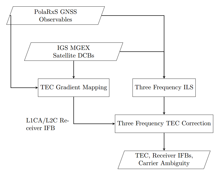
We can remove satellite IFB using estimates from IGS
\Delta b_{S,f_i,f_j}
We express ionosphere delays in terms of TEC
\Delta ADR_{f_i,f_j} \approx \Delta b_{R,f_i,f_j} - \frac{40.3\times 10^{16}}{\alpha_{f_i,f_j}}TEC
+ \lambda_{f_i} N_{S,f_i} - \lambda_{f_j} N_{S,f_j} + \cdots
CMC_f \approx \frac{40.3\times 10^{16}}{f^2}TEC - \lambda_f N_{S,f} + \cdots
multipath / noise / unmodeled errors
ILS TEC Estimation
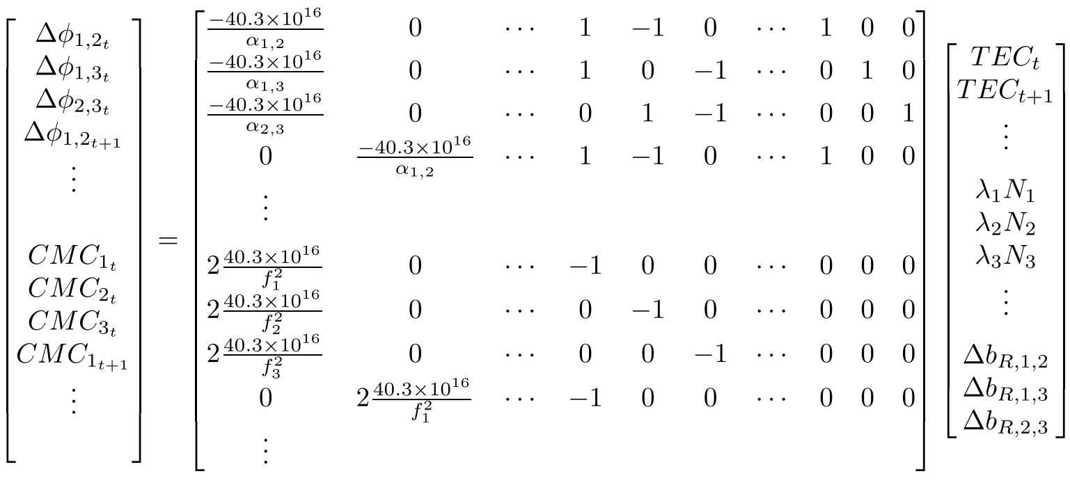
Use iterative least-squares to solve large sparse system for 1 day of data
Experiment Data
GPS Lab high-rate GNSS data collection network
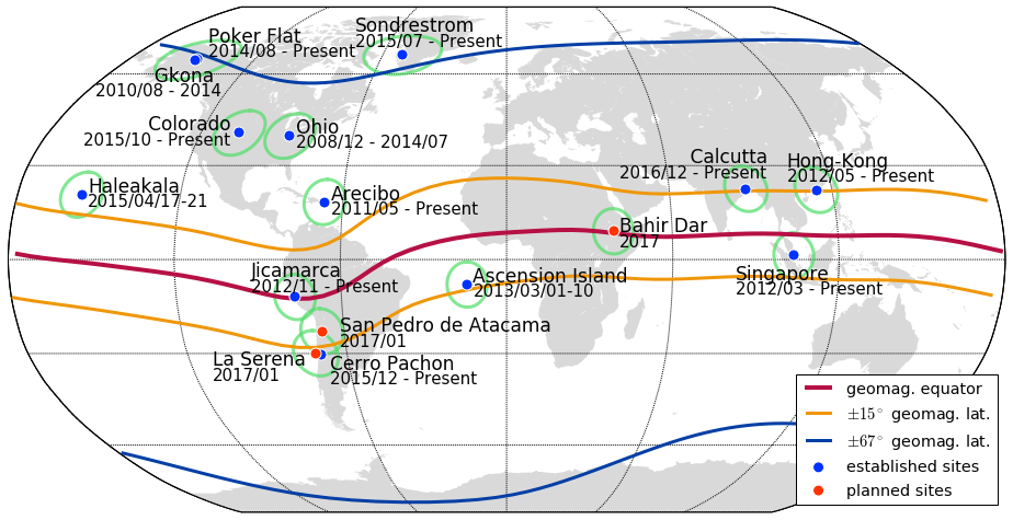
- 3-receiver array near Poker Flat, Alaska
- 2016 / 04 / 15
- Septentrio PolarXs
- 1 Hz GPS L1/L2/L5 measurements
TEC Leveling
Estimated TEC is too low due to direct trade-off between TEC and IFB biases
Some ionosphere constraint or model must be imposed in order to estimate actual IFB
vTEC Gradient-Mapping Method
Assume ionosphere vertical TEC can be described by a linear 2D gradient near receiver
Solve sparse linear system of code-minus-carrier and ADR difference observables
See Harrison Bourne thesis (2016)
vTEC
TEC
delta lat/lon
Method Summary
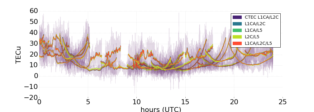
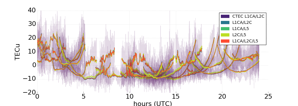
Results
2016 / 04 / 30 - Antenna 1
Full day summary shows physically reasonable TEC levels
Results
Results
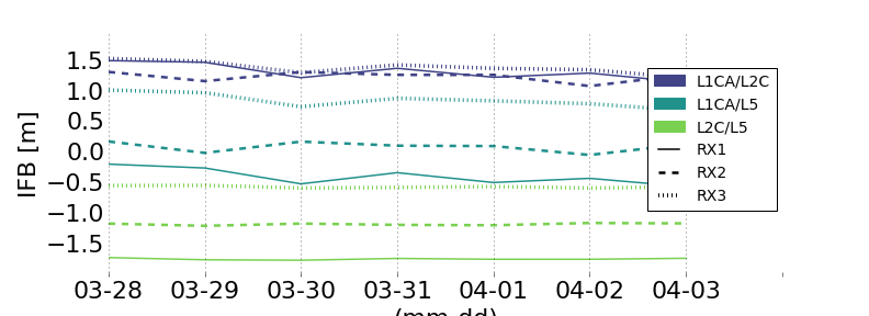
Shows relatively stable receiver IFBs over 7 days
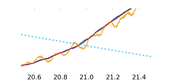
Results
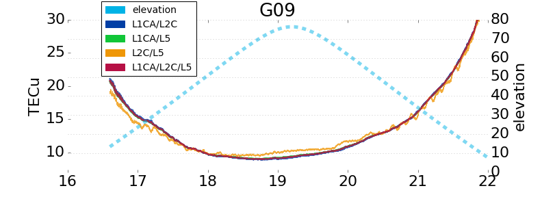
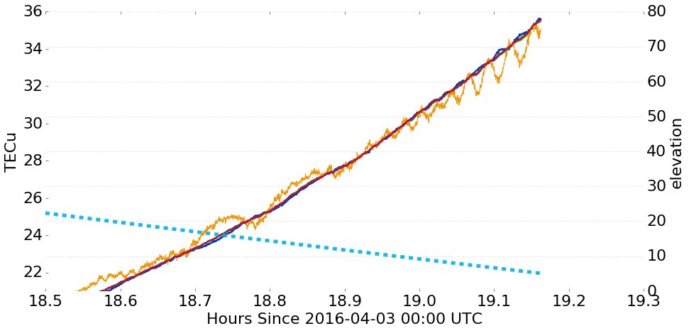
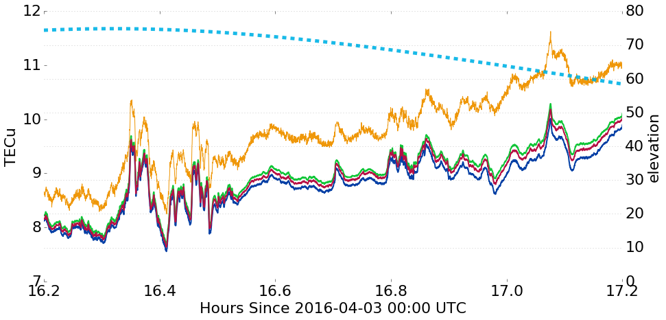
PRN 08 showing high-elevation structure
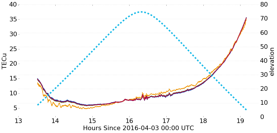
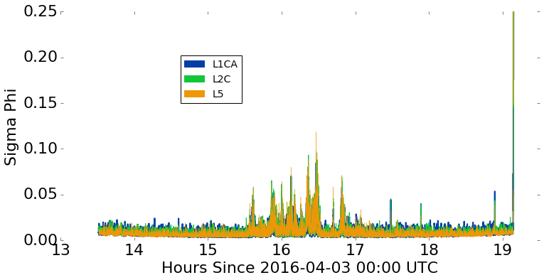
Results
(close-ups of previous slide)
Conclusions
- demonstrated method to estimate TEC, receiver IFBs, and carrier ambiguities using 3-frequency GPS signals
- vTEC Gradient-Mapping method was used as the ionosphere constraint in order to receiver IFB bias
- TEC appears leveled to physically reasonable values
- receiver IFBs appear stable over several days
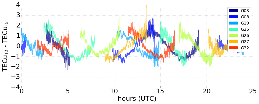
- algorithm is useful for first-step analysis into the origin of remaining errors between TEC computed using 2 frequencies
Future Work
What causes errors?
- satellite pass / geometry
- antenna azimuth effects
- phase wind-up
- ???
Acknowledgements
This research was supported by the Air Force Research Laboratory and NASA.
References
Spits, Justine. Total Electron Content reconstruction using triple frequency GNSS signals. Diss. Université de Liège, Belgique, 2012.
Bourne, Harrison W. An algorithm for accurate ionospheric total electron content and receiver bias estimation using GPS measurements. Diss. Colorado State University. Libraries, 2016.
Improved Estimation of Ionosphere TEC Using Triple-Frequency GPS Signals
By Brian Breitsch


