Long-Term Analysis of Carrier Phase Residual Variations
Brian Breitsch
Jade Morton
Charles Rino

Using Geometry-Ionosphere-Free Combination of Triple-Frequency GPS Observations
ION GNSS 2017
Background and Motivation
Linear Estimation of GNSS Parameters
Application to Real GPS Data
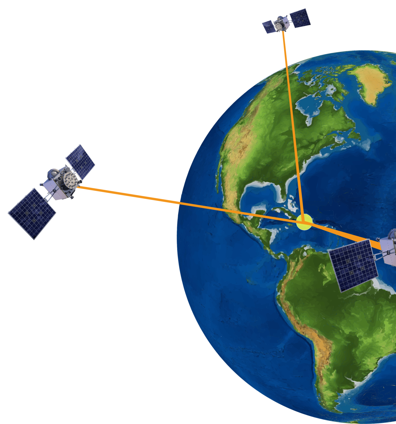
Global Navigation Satellite Systems (GNSS)
...a useful everyday radio source for geophysical remote-sensing!
GPS
GLONASS
Beidou
Galileio
...etc.
GPS - Global Positioning System
- 32-satellite constellation
- transmit dual-frequency BPSK-moduled signals
| Signal | Frequency (GHz) |
|---|---|
| L1CA | 1.57542 |
| L2C | 1.2276 |
| L5 | 1.17645 |

- new Block-IIF and next-gen
Block-III satellites transmitting triple-frequency signals
GNSS Carrier Phase Observable
\Phi_i = r + c\Delta t + T + I_i + \lambda_i N_i + H_i + S_i + \epsilon_i
HARDWARE BIAS
IONOSPHERE RANGE ERROR
CARRIER AMBIGUITY
SYSTEMATIC ERRORS / MULTIPATH
FREQUENCY INDEPENDENT EFFECTS
STOCHASTIC ERRORS
accumulated phase (in meters) of demodulated GNSS signal at receiver for a particular satellite and signal carrier frequency \(f_i\)
Simplified Carrier Phase Model
\Phi_i = G + I_i + S_i + \epsilon_i
zero-mean
normally-
distributed
zero-mean
neglect bias terms
By neglecting bias terms, we address estimation precision, rather than accuracy
\Phi_i = r + c\Delta t + T + I_i + \lambda_i N_i + H_i + S_i + \epsilon_i
"geometry" term
Ionosphere Range Error
consider first-order term in ionosphere refractive index
second and higher-order terms on the order of a few cm
I_i
\approx -\frac{\kappa}{f_i^2} \displaystyle \int_\text{rx}^\text{tx} N_e \ ds = -\frac{\kappa}{f_i^2} \text{TEC}
\kappa = \frac{e^2}{8\pi^2\epsilon_0 m_e} \approx 40.301
TOTAL ELECTRON CONTENT

rx
tx
plasma / free electrons
units: \(\frac{\text{electrons}}{\text{m}^2}\)
often measured in TEC units:
1 \text{TECu} = 10^{16} \frac{\text{electrons}}{\text{m}^2}
f_i
carrier frequency
Estimation of \(G\) and \(\text{TEC}\) Using Dual-Frequency GNSS
neglecting systematic and stochastic error terms, and after resolving bias terms:
\text{TEC} = \displaystyle \frac{\Phi_2 - \Phi_1}{\kappa \left(\frac{1}{f_1^2} - \frac{1}{f_2^2}\right)}
G = \displaystyle \frac{f_1^2 \Phi_1 - f_2^2 \Phi_2}{f_1^2 - f_2^2}
ionosphere-free combination
geometry-free combination
Examples of Dual-Frequency TEC Estimates

Poker Flat, Alaska, 2016-01-02
We compute dual-frequency TEC estimates \(\text{TEC}_\text{L1,L2}\) and \(\text{TEC}_\text{L1,L5}\)
\(G_{\text{L1,L5}} - G_{\text{L1,L2}} = \text{TEC}_{\text{L1,L5}} - \text{TEC}_{\text{L1,L2}}\)
Poker Flat, Alaska, 2016-01-02

Can we characterize / find the source of these discrepancies?
Can we relate them to errors in range and TEC estimates?
Background and Motivation
Linear Estimation of GNSS Parameters
Application to Real GPS Data
model parameters
\mathbf{\Phi} = \left[\Phi_1, \cdots, \Phi_m\right]^T
\mathbf{m} = \left[G, \text{TEC}, S_1, \cdots, S_m \right]^T
\mathbf{A} = \begin{bmatrix}
1 & -\frac{\kappa}{f_1^2} & 1 & 0 & \cdots & 0 \\
1 & -\frac{\kappa}{f_2^2} & 0 & 1 & \cdots & 0 \\
\vdots & & & & \ddots & \\
1 & -\frac{\kappa}{f_m^2} & 0 & \cdots & & 1
\end{bmatrix}
\mathbf{\epsilon} = [\epsilon_1, \cdots, \epsilon_m]^T
\mathbf{\Phi} = \mathbf{A} \mathbf{m} + \mathbf{\epsilon}
Linear Inverse Problem
observations
stochastic error
forward model
Linear Estimation
\mathbf{\hat{m}} \approx \mathbf{A^*} \mathbf{\Phi}
We must apply a priori information about model parameters
\mathbf{A^*} =\begin{bmatrix}
\mathbf{C}_G \\
\mathbf{C}_\text{TEC} \\
\mathbf{C}_{S_1} \\
\vdots \\
\mathbf{C}_{S_m}
\end{bmatrix}
geometry estimator
TECu estimator
systematic-error estimators
|G| , |I_i| \gg |S_i|
G \sim
I \sim
S \sim
20,000 km
1 - 150 m
several cm
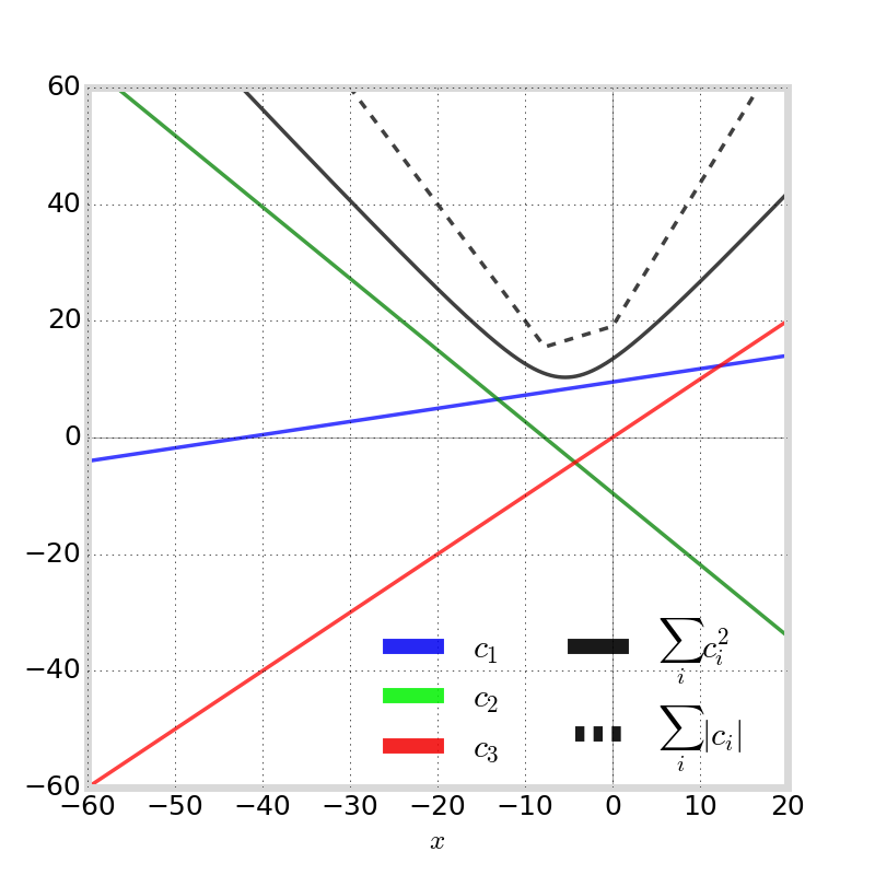
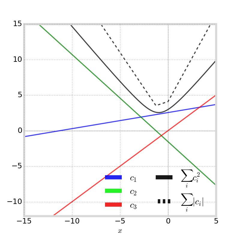
Linear Coefficient Constraints
Use one or two of the following constraints to reduce search space for optimal estimator coefficients:
\sum_i c_i = 0
\sum_i c_i = 1
geometry-free
geometry-estimator
\sum_i -\frac{\kappa}{f_i^2}c_i = 1
\sum_i \frac{c_i}{f_i^2} = 0
TEC-estimator
ionosphere-free
\Phi_i = G + I_i + S_i + \epsilon_i
Reduction of Error
\mathbf{C}^* = \ \displaystyle \arg\min_\mathbf{C} \mathbf{C}^T \Sigma_\epsilon \mathbf{C}
Linear combination stochastic error variance:
\sigma_\epsilon^2 = \mathbf{C}^T \mathbf{\Sigma}_\epsilon \mathbf{C}
where \(\mathbf{\Sigma}_\epsilon\) is the covariance matrix between \(\mathbf{\epsilon}_i\)
Optimal \(\mathbf{C}\) for minimizing stochastic error variance:
\(\epsilon_i\) equal-amplitude and uncorrelated
\mathbf{C}^* = \ \displaystyle \arg\min_\mathbf{C} \sum_i c_i^2
TEC Estimator
1. apply TEC-estimator constraint
2. apply geometry-free constraint (since \(|G| \gg |I_i|\) )
Dual-Frequency Example
\Rightarrow c_1 = \displaystyle -\frac{1}{\kappa \left(\frac{1}{f_1^2} - \frac{1}{f_2^2}\right)}
\begin{aligned}
& -\frac{\kappa}{f_1^2}c_1 - \frac{\kappa}{f_2^2}c_2 = 1 \\[1em]
& c_1 + c_2 = 0 \Rightarrow c_1 = -c_2 \\[1em]
\Rightarrow & -\kappa c_1 \left(\frac{1}{f_1^2} - \frac{1}{f_2^2}\right) = 1
\end{aligned}
TEC-estimator
geometry-free
recall:
\text{TEC} = \displaystyle \frac{\Phi_2 - \Phi_1}{\kappa \left(\frac{1}{f_1^2} - \frac{1}{f_2^2}\right)}
Triple-Frequency TEC Estimator

Applying constraints yields following system of coefficients (with free parameter denoted \(x\):
\begin{aligned}
c_1 &= \frac{\frac{1}{\kappa} + x \left( \frac{1}{f_3^2} - \frac{1}{f_2^2}\right)}{\frac{1}{f_2^2} - \frac{1}{f_1^2}} \\[1em]
c_2 &= \frac{-\frac{1}{\kappa} - x \left( \frac{1}{f_3^2} - \frac{1}{f_1^2}\right)}{\frac{1}{f_2^2} - \frac{1}{f_1^2}}
\\[1em]
c_3 & = \ \ x
\end{aligned}
x^* = \frac{\frac{1}{\kappa}\left(\frac{2}{f_3^2} - \frac{1}{f_2^2} - \frac{1}{f_1^2}\right)}{\left(\frac{1}{f_1^2} - \frac{1}{f_2^2}\right)^2 + \left(\frac{1}{f_2^2} - \frac{1}{f_3^2}\right)^2 + \left(\frac{1}{f_3^2} - \frac{1}{f_1^2}\right)^2}
To satisfy \( \mathbf{C}^* = \ \displaystyle \arg\min_\mathbf{C} \sum_i c_i^2 \), choose
denote corresponding coefficient vector \(\mathbf{C}_{\text{TEC}_{1,2,3}}\) and its corresponding estimate \(\text{TEC}_{1,2,3}\)
TEC Estimator Using Triple-Frequency GPS

\begin{matrix}
\text{Estimate} & c_1 & c_2 & c_3 & \sum_i c_i^2 \\[.5em]
\text{TEC}_\text{L1,L2,L5} & 8.294 & -2.883 & -5.411 & 10.314 & \\
\text{TEC}_\text{L1,L5} & 7.762 & 0 & -7.762 & 10.977 & \\
\text{TEC}_\text{L1,L2} & 9.518 & -9.518 & 0 & 13.460 & \\
\text{TEC}_\text{L2,L5} & 0 & 42.080 & -42.080 & 59.510 &
\end{matrix}
\mathbf{C}_{\text{TEC}_\text{L1,L2,L5}}
\mathbf{C}_{\text{TEC}_\text{L1,L5}}
\mathbf{C}_{\text{TEC}_\text{L1,L2}}
\mathbf{C}_{\text{TEC}_\text{L2,L5}}
Geometry Estimator
\begin{matrix}
c_1 = & \frac{-\frac{1}{f_2^2} + x \left(\frac{1}{f_2^2} - \frac{1}{f_3^2}\right)}{\frac{1}{f_1^2} - \frac{1}{f_2^2}} \\
c_2 = & \frac{\frac{1}{f_1^2} - x \left(\frac{1}{f_1^2} - \frac{1}{f_3^2}\right)}{\frac{1}{f_1^2} - \frac{1}{f_2^2}} \\
c_3 = & x
\end{matrix}
For triple-frequency GNSS:
1. apply geometry-estimator constraint
2. apply ionosphere-free constraint since \(I_i\) are the next-largest terms
x^* = \frac{\frac{1}{\kappa}\left(\frac{2}{f_3^2} - \frac{1}{f_2^2} - \frac{1}{f_1^2}\right)}{\left(\frac{1}{f_1^2} - \frac{1}{f_2^2}\right)^2 + \left(\frac{1}{f_2^2} - \frac{1}{f_3^2}\right)^2 + \left(\frac{1}{f_3^2} - \frac{1}{f_1^2}\right)^2}
To satisfy \( \mathbf{C}^* = \ \displaystyle \arg\min_\mathbf{C} \sum_i c_i^2 \),
We call this coefficient vector \(\mathbf{C}_{G_{1,2,3}}\) and its corresponding estimate \(G_{1,2,3}\)
the optimal "ionosphere-free combination"
Geometry Estimator Using Triple-Frequency GPS
\begin{matrix}
\text{Estimate} & c_1 & c_2 & c_3 & \sum_i c_i^2 \\[.5em]
G_\text{L1,L2,L5} & 2.327 & -0.360 & -0.967 & 2.546 \\
G_\text{L1,L5} & 2.261 & 0 & -1.261 & 2.588 \\
G_\text{L1,L2} & 2.546 & -1.546 & 0 & 2.978 \\
G_\text{L2,L5} & 0 & 12.255 & -11.255 & 16.639
\end{matrix}

\mathbf{C}_{G_\text{L1,L2,L5}}
\mathbf{C}_{G_\text{L1,L5}}
\mathbf{C}_{G_\text{L1,L2}}
\mathbf{C}_{G_\text{L2,L5}}
Systematic Error Estimator
Since \(|G| \gg |I_i| \gg |S_i|\), must apply both geometry-free and ionosphere-free constraints
For triple-frequency GNSS:
\begin{aligned}
c_1 & = \ \ x \frac{\frac{1}{f_3^2} - \frac{1}{f_2^2}}{\frac{1}{f_2^2} - \frac{1}{f_1^2}} \\[1em]
c_2 & = - x \frac{\frac{1}{f_3^2} - \frac{1}{f_1^2}}{\frac{1}{f_2^2} - \frac{1}{f_1^2}} \\[1em]
c_3 & = \ \ x
\end{aligned}
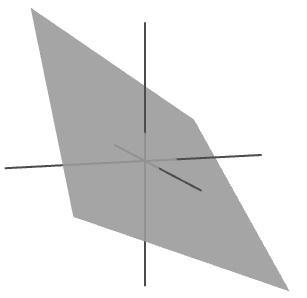
system is linear subspace
there is "only one" estimate of systematic errors
note this requires \(m \ge 3\)

Geometry-Ionosphere-Free Combination
FACT: The difference between any two geometry term or any two TEC estimates produces some scaling of the GIFC
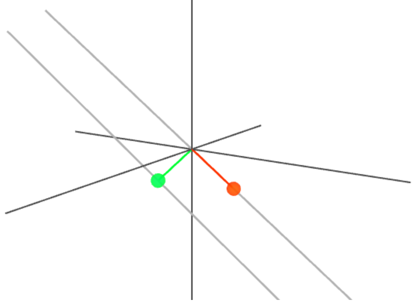
FACT: \(\mathbf{C}_\text{GIFC} \perp \mathbf{C}_{G_{1,2,3}}\) and \(\mathbf{C}_\text{GIFC} \perp \mathbf{C}_{\text{TEC}_{1,2,3}}\)
\mathbf{C}_{\text{TEC}_{1,2,3}}
\mathbf{C}_\text{GIFC}
information about systematic and stochastic errors present in GNSS carrier phase observables
GIFC Triple-Frequency GPS
\begin{aligned}
\mathbf{C}_{\text{GIFC}_\text{L1,L2,L5}} & = \mathbf{C}_{\text{TEC}_{\text{L1,L5}}} - \mathbf{C}_{\text{TEC}_{\text{L1,L2}}} \\[1em]
& = \left[-1.756, 9.520, -7.764\right]^T
\end{aligned}
We (arbitrarily) choose:
Note: the triple-frequency GIFC does not have a well-defined unit.
GIFC in our results section have the scaling shown here.
Background and Motivation
Linear Estimation of GNSS Parameters
Application to Real GPS Data
Experiment Data
GPS Lab high-rate GNSS data collection network
- Alaska, Hong Kong, Peru
- 2013, 2014, 2015, 2016
- 1 Hz GPS L1/L2/L5 measurements
- Septentrio PolarXs

GIFC Examples


Peru G24
Hong Kong G24
Peru G25
Alaska G01
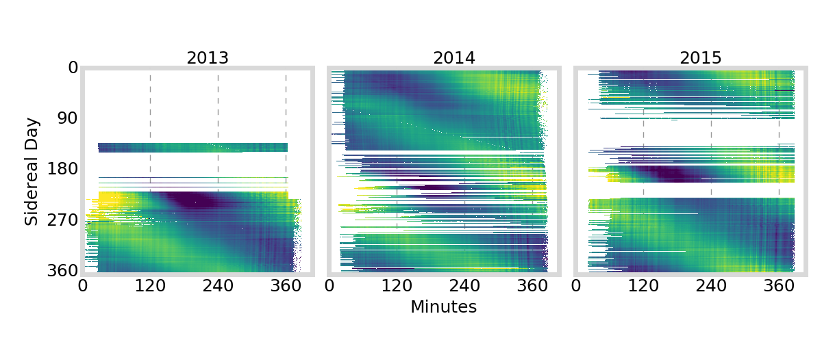

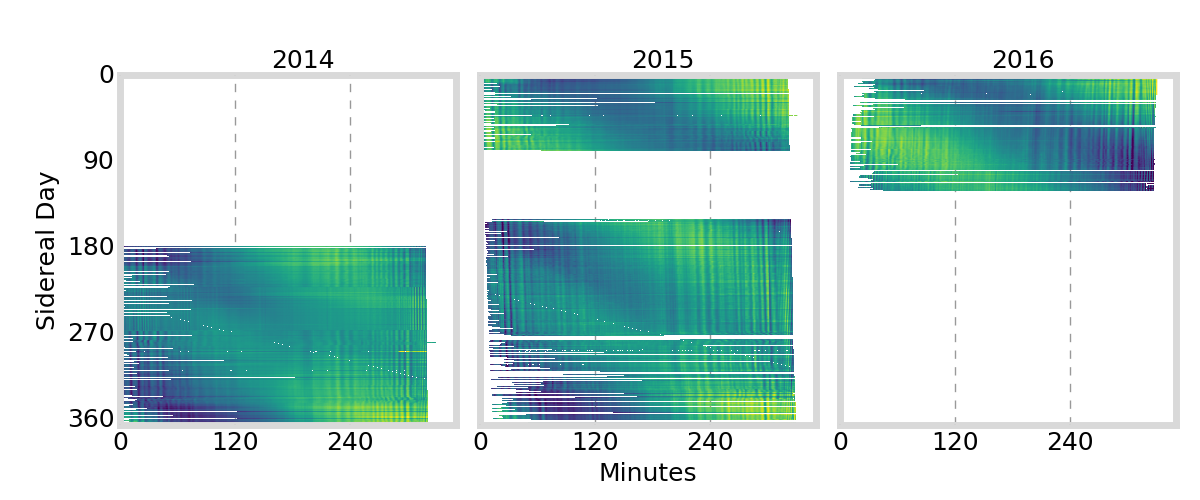


GIFC Calendar
Hong Kong G24
Alaska G25
Alaska G01

- large, long-term GIFC trend likely due mostly to satellite thermal oscillations
- studied by (Montebruck et. al. 2012) and (Li et. al. 2013)
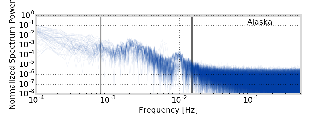


GIFC Spectrum
Alaska
Hong Kong
Peru


GIFC Histogram
Peru Example

Conclusions
- GIFC is an indicator of the presence of systematic / stochastic errors
- two main components to GIFC
- large, low-frequency trend (likely due to satellite thermal oscillations)
- multipath
- this work is a step towards improved assessment of precision of GNSS phase-related estimates, particularly ionosphere TEC
- small improvement of triple-frequency estimators over dual-frequency signal pair with widest frequency separation
References
O. Montenbruck, U. Hugentobler, R. Dach, P. Steigenberger, and A. Hauschild, “Apparent clock variations of the Block IIF-1 (SVN62) GPS satellite,” GPS Solutions, vol. 16, no. 3, pp. 303–313, 2012.
H. Li, X. Zhou, and B. Wu, “Fast estimation and analysis of the inter-frequency clock bias for Block IIF satellites,” GPS Solutions, vol. 17, no. 3, pp. 347–355, 2013.
Acknowledgements
This research was supported by the Air Force Research Laboratory and NASA.
ION GNSS 2017 - Information From Multi-Frequency GNSS
By Brian Breitsch


