Analysis of Carrier Phase Residual Trend Variations
Brian Breitsch\(^1\)
Jade Morton\(^1\)
Using the Geometry-Ionosphere-Free Combination
SAINT Update 2017
1. University of Colorado Boulder
Motivation:
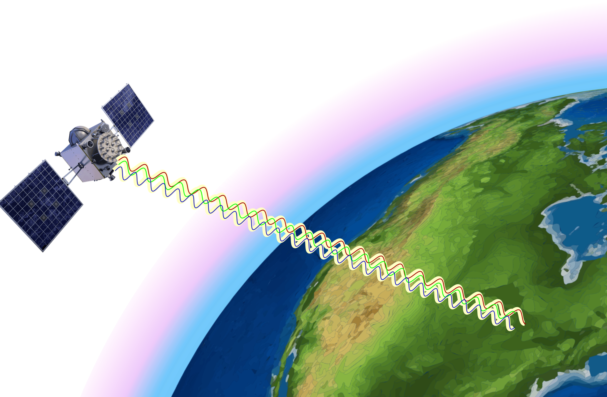
TEC and Triple-Frequency
Background:
Linear Estimation of GNSS Parameters
Main Topic:
Geometry-Ionosphere-Free Combination
Analysis and Results:
GIFC From Real GPS Data
Motivation:
TEC and Triple-Frequency
Background:
Linear Estimation of GNSS Parameters
Main Topic:
Geometry-Ionosphere-Free Combination
Analysis and Results:
GIFC From Real GPS Data
Carrier Phase and TEC

\Phi_i = r + c\Delta t + T + I_i + \lambda_i N_i + H_i + S_i + \epsilon_i
HARDWARE BIASES
IONOSPHERE RANGE ERROR
CARRIER AMBIGUITY
SYSTEMATIC ERRORS / MULTIPATH
FREQUENCY INDEPENDENT EFFECTS
STOCHASTIC ERRORS
frequency \(f_i\)
I_i \approx -\frac{\kappa}{f_i^2} \text{TEC}
plasma / free electrons

Multi-Frequency GNSS
- GPS Block IIF / Block III
- Galileo (E1, E5a/b)
- GLONASS-K2
| Signal | Frequency (GHz) |
|---|---|
| L1CA | 1.57542 |
| L2C | 1.2276 |
| L5 | 1.17645 |
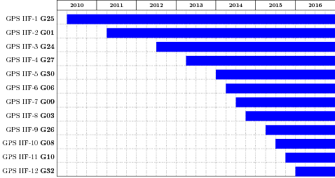
triple-frequency GPS
12 satellites since 2016
Estimation of \(G\) and \(\text{TEC}\) Using Dual-Frequency GNSS
\text{TEC} = \displaystyle -\frac{\Phi_1 - \Phi_2}{\kappa \left(\frac{1}{f_1^2} - \frac{1}{f_2^2}\right)}
G = \displaystyle \frac{f_1^2 \Phi_1 - f_2^2 \Phi_2}{f_1^2 - f_2^2}
ionosphere-free combination
geometry-free combination
\Phi_i = G + I_i + S_i + \epsilon_i
"geometry" term
\Phi_i = r + c\Delta t + T + I_i + \lambda_i N_i + H_i + S_i + \epsilon_i
we can solve bias terms
Examples of Two Dual-Frequency TEC Estimates
Poker Flat, Alaska, 2016-01-02
Can we characterize / find the source of these discrepancies?

Motivation:
TEC and Triple-Frequency
Background:
Linear Estimation of GNSS Parameters
Main Topic:
Geometry-Ionosphere-Free Combination
Analysis and Results:
GIFC From Real GPS Data
model parameters
\mathbf{\Phi} = \left[\Phi_1, \cdots, \Phi_m\right]^T
\mathbf{m} = \left[G, \text{TEC}, S_1, \cdots, S_m \right]^T
\mathbf{\Phi} = \mathbf{A} \mathbf{m} + \mathbf{\epsilon}
Linear Inverse Problem
observations
\Phi_i = G + I_i + S_i + \epsilon_i
\mathbf{\hat{m}} \approx \mathbf{A^*} \mathbf{\Phi}
estimate:
\mathbf{A^*} =\begin{bmatrix}
\mathbf{C}_G \\
\mathbf{C}_\text{TEC} \\
\mathbf{C}_{S_1} \\
\vdots \\
\mathbf{C}_{S_m}
\end{bmatrix}
geometry estimator
TEC estimator
systematic-error estimators
Linear Coefficient Constraints
\sum_i c_i = 0
\sum_i c_i = 1
geometry-free
geometry-estimator
\sum_i -\frac{\kappa}{f_i^2}c_i = 1
\sum_i \frac{c_i}{f_i^2} = 0
TEC-estimator
ionosphere-free
\Phi_i = G + I_i + S_i + \epsilon_i
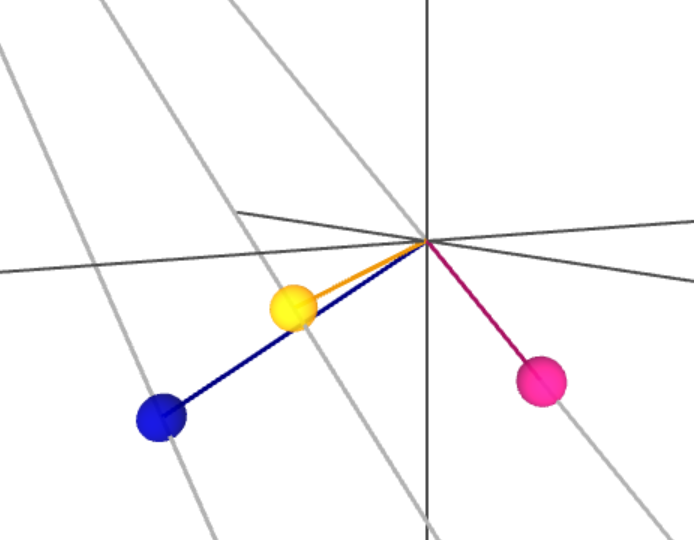
solutions at intersection of constraint hyperplanes

|G| , |I_i| \gg |S_i|
a-priori information:
Estimators
\(\text{TEC}\) Estimator
TEC-estimator + geometry-free constraints
\(G\) Estimator
geometry-estimator + ionosphere-free constraints
\(\text{L1,L2,L5}\)
\(\text{L1,L5}\)
\(\text{L1,L2}\)


choose min-norm
Triple-Frequency GPS Estimator Coefficients
\begin{matrix}
\text{Estimate} & c_1 & c_2 & c_3 & \text{noise amp.} \\[.5em]
G_\text{L1,L2,L5} & 2.3 & -0.4 & -1.0 & 2.5 \\
G_\text{L1,L5} & 2.3 & 0 & -1.3 & 2.6 \\
G_\text{L1,L2} & 2.5 & -1.5 & 0 & 3.0 \\
G_\text{L2,L5} & 0 & 12.3 & -11.3 & 16.6
\end{matrix}
\begin{matrix}
\text{Estimate} & c_1 & c_2 & c_3 & \text{noise amp.} \\[.5em]
\text{TEC}_\text{L1,L2,L5} & 8.3 & -2.9 & -5.4 & 10.3 & \\
\text{TEC}_\text{L1,L5} & 7.8 & 0 & -7.8 & 11.0 & \\
\text{TEC}_\text{L1,L2} & 9.5 & -9.5 & 0 & 13.5 & \\
\text{TEC}_\text{L2,L5} & 0 & 42.1 & -42.1 & 59.5 &
\end{matrix}
\(G\) Estimator
\(\text{TEC}\) Estimator
Triple-Frequency TEC Estimate Examples


Motivation:
TEC and Triple-Frequency
Background:
Linear Estimation of GNSS Parameters
Main Topic:
Geometry-Ionosphere-Free Combination
Analysis and Results:
GIFC From Real GPS Data
Estimating Systematic Errors
apply both geometry-free and ionosphere-free constraints
For triple-frequency GNSS:
\begin{aligned}
c_1 & = \ \ x \frac{\frac{1}{f_3^2} - \frac{1}{f_2^2}}{\frac{1}{f_2^2} - \frac{1}{f_1^2}} \\[1em]
c_2 & = - x \frac{\frac{1}{f_3^2} - \frac{1}{f_1^2}}{\frac{1}{f_2^2} - \frac{1}{f_1^2}} \\[1em]
c_3 & = \ \ x
\end{aligned}
system is linear subspace
there is "only one estimate" of systematic errors
note this requires \(m \ge 3\)

\Phi_i = G + I_i + S_i + \epsilon_i
Geometry-Ionosphere-Free Combination
\mathbf{C}_{\text{TEC}_{1,2,3}}
\mathbf{C}_\text{GIFC}
information about systematic and stochastic errors present in GNSS carrier phase observables
\begin{aligned}
\mathbf{C}_{\text{GIFC}_\text{L1,L2,L5}} & = \mathbf{C}_{\text{TEC}_{\text{L1,L5}}} - \mathbf{C}_{\text{TEC}_{\text{L1,L2}}} \\[1em]
& = \left[-1.756, \ 9.520, \ -7.764\right]
\end{aligned}
We (arbitrarily) choose:
\Phi_i = G + I_i + S_i + \epsilon_i
\mathbf{C}_{G_{1,2,3}}
\( \text{GIFC} = G_{1,3} - G_{1,2} \)
\( \text{GIFC} = \text{TEC}_{1,3} - \text{TEC}_{1,2} \)
Motivation:
TEC and Triple-Frequency
Background:
Linear Estimation of GNSS Parameters
Main Topic:
Geometry-Ionosphere-Free Combination
Analysis and Results:
GIFC From Real GPS Data
Experiment Data
Sense Lab high-rate GNSS data collection network
- Alaska, Hong Kong, Peru
- 2013 - 2016
- 1 Hz GPS L1/L2/L5 measurements
- Septentrio PolarXs

GIFC Examples
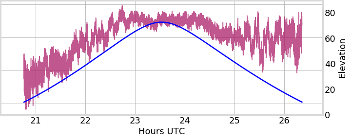
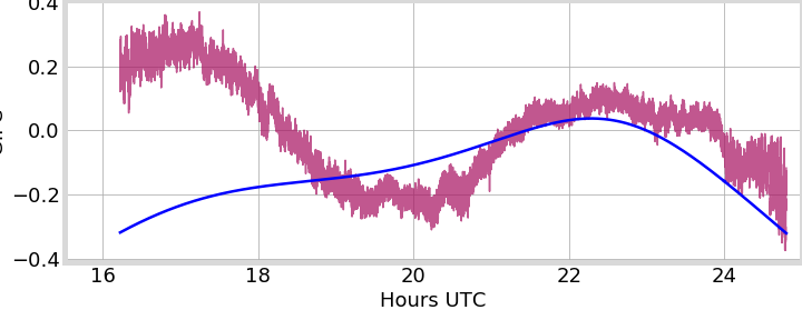
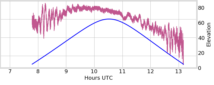
PRN 24, Peru
PRN 24, Hong Kong
PRN 25, Peru
PRN 01, Alaska
2013-01-01
2014-05-15
2013-01-01
2014-06-29
GIFC
Sat. Elevation


GIFC Calendar
PRN 24, Hong Kong
PRN 25, Hong Kong
PRN 24, Alaska

PRN 25, Alaska
GIFC Calendar
PRN 25, Alaska
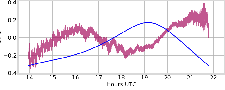
- large, long-term GIFC trend likely due mostly to satellite thermal oscillations
- studied by (Montebruck et. al. 2012) and (Li et. al. 2013)


\(\theta\)


GIFC Histogram
Peru Example
estimate trend \(\Rightarrow\) reduce major component of TEC and G estimate errors
(all satellites, all data)
Conclusions
- GIFC is an indicator of the presence of systematic / stochastic errors
- dominant GIFC component is periodic
- long, arc-wide trend due to satellite thermal variations
- errors on order of up to 0.5 TECu
- need to start estimating variable IFB corrections to accommodate TEC / geometry estimates
Next Steps
- use to analyze other systematic dispersive errors such as multipath and strong scintillation
References
O. Montenbruck, U. Hugentobler, R. Dach, P. Steigenberger, and A. Hauschild, “Apparent clock variations of the Block IIF-1 (SVN62) GPS satellite,” GPS Solutions, vol. 16, no. 3, pp. 303–313, 2012.
H. Li, X. Zhou, and B. Wu, “Fast estimation and analysis of the inter-frequency clock bias for Block IIF satellites,” GPS Solutions, vol. 17, no. 3, pp. 347–355, 2013.
B. Breitsch, "Optimal Linear Combinations of GNSS Phase Observables to Improve and Assess TEC Estimation Precision," Masters Thesis, Colorado State University
Acknowledgements
This research was supported by the Air Force Research Laboratory.
SAINT Update - Analysis of Carrier Phase Residual Using Geometry-Ionosphere-Free Combination of Triple-Frequency GPS Observations
By Brian Breitsch


